Chapter 15
Feature Selection & Dimensionality Reduction
Feature engineering fills a dataset with columns. This chapter is about admitting that not all of them are useful. One-hot encoding, interaction terms, datetime extraction: you’ve done it all. A modelling table can carry hundreds of columns. Past a point, more columns stop helping and start hurting. Models overfit. Training slows. Distance-based methods stop behaving sensibly. Two different operations both go by the name “dimensionality reduction,” which invites confusion rather than avoiding it. Feature selection keeps a subset of the original columns, so “income” stays income. Feature extraction builds a smaller number of new columns that are blends of the originals, trading interpretability for compactness. Both exist to fight the same enemy: the curse of dimensionality. Knowing which one a given situation needs matters as much as knowing how to run either.
15.1 Motivation
Chapter 14’s feature engineering deliberately produces more candidate columns than a model needs. The theory is that it’s cheaper to generate too much signal and prune it than to under-engineer and miss something. That pruning step is this chapter. Without it, a model trained on hundreds of largely redundant or irrelevant features doesn’t just run slower. It performs worse. It has more surface area on which to fit noise instead of signal. The goal is a feature set that is as small as it can be, without discarding anything that helps. Get there by keeping the best of what already exists (selection), or by compressing everything into fewer, denser dimensions (extraction).
15.2 Exposition
15.2.1 The Curse of Dimensionality
Three things get worse as the number of features grows. Distances stop being informative. In high dimensions, the ratio between the nearest and farthest neighbour’s distance shrinks towards 1. “Nearest” stops meaning much for the algorithms that depend on it: KNN, K-Means, anything built on Euclidean or cosine similarity. The data becomes sparse relative to the space. Keeping the same density of training examples per unit volume requires the number of examples to grow exponentially with the number of dimensions. With 20 features and a modest sample size, the data is a thin cloud in a mostly empty 20-dimensional space. Overfitting risk rises. More features means more ways to fit noise rather than signal, especially with a fixed number of rows. 500 features and 1,000 rows gives a model enormous freedom to memorise the training set rather than learn from it. There’s also a practical cost, independent of any statistical concerns: more features means more compute, more memory, and slower training.
The sparsity claim is easy to say and easy to underestimate, so it’s worth making concrete with numbers. Picture a cube of jelly, one unit of length on each side, with a million tiny balls suspended in it. One ball per data point. Say the cube has 3 dimensions: three features, each ranging over that unit of length. A million evenly-spaced balls sit roughly of the cube’s side apart from their nearest neighbours. That’s close enough that “nearest” means something. Now stretch that same cube into 20 dimensions. One axis per feature. Keep the same million balls. The average spacing between a ball and its nearest neighbour becomes : roughly half the entire length of the cube’s side. The same million points that felt dense in 3 dimensions are, in 20 dimensions, spread so thinly that each point’s nearest neighbour is half the cube away. No amount of data collection closes that gap. Matching the 3-dimensional spacing of in 20 dimensions would need balls, about times the million we started with. This is the curse. Adding dimensions doesn’t make a dataset a little sparser. It makes it exponentially, catastrophically sparser, for a fixed number of examples.
15.2.2 Feature Selection: Filter, Wrapper, Embedded
Selection methods fall into three families, distinguished by how they decide which features matter.
Filter methods score each feature independently of any model, then keep the top scorers:
- Variance threshold drops near-constant features, which carry no signal for any model.
- Correlation with the target keeps features most linearly related to
y. It’s cheap but blind to non-linear relationships, so a feature with a perfect U-shaped relationship to the target scores near-zero linear correlation and gets wrongly discarded. - Mutual information measures any dependency, linear or not, between a feature and the target. Slower than correlation, but far more reliable at catching non-linear signal.
Filters are fast (score everything once, sort, cut) but they ignore how features interact with each other and with whatever model will consume them.
Wrapper methods use the downstream model’s own performance to decide what to keep, searching over subsets directly rather than scoring features in isolation. Recursive Feature Elimination (RFE) trains the model, ranks features by importance or coefficient magnitude, drops the weakest, and repeats until reaching a target count. This directly optimises for what matters: model performance. But it’s expensive. It retrains the model repeatedly. And the resulting subset is specific to whichever model did the selecting.
Embedded methods get selection for free as a side effect of training a model that has sparsity or importance built in. L1 regularisation (Lasso) drives some coefficients exactly to zero, building selection into the loss function (Chapter 18 covers regularisation in depth). Tree-based importances (Random Forest, gradient-boosted trees) naturally produce a feature ranking as a byproduct of how often and how effectively each feature was used for splitting. Embedded methods are usually the best default in practice: they give selection signal without a separate search loop. But the importance scores can be biased towards high-cardinality or correlated features. Treat them as a hint, nothing more.
15.2.3 Feature Extraction: PCA
Principal Component Analysis doesn’t select features. It constructs new ones. The idea: find the direction in feature space along which the data varies most, call that the first principal component. Find the next direction (orthogonal to the first) that captures the most remaining variance. Repeat. Mathematically this is an eigendecomposition of the feature covariance matrix. If is the covariance matrix of the standardised features, PCA finds its eigenvectors and eigenvalues:
Each eigenvector is a principal component (a direction in feature space) and its eigenvalue is the amount of variance captured along that direction. Sorting components by eigenvalue, largest first, and keeping the top gives the -dimensional linear subspace that preserves the most variance possible for that value of . In practice, a dataset almost never needs every original dimension to explain the bulk of its variance. Ten correlated features might contain only three or four independent “directions” of information. PCA finds them.
Standardise features before applying PCA. Variance is scale-dependent, and PCA chooses directions of maximum variance. A feature measured in dollars (range: thousands) will dominate the variance calculation over one measured in years (range: tens), purely because of its scale, not because it’s more informative. There are no right answers here, only trade-offs. With PCA the trade-off is interpretability. Component 1 is something like : a blend rather than a concept. Say a prediction needs to be explained in terms of a specific original variable, for a regulator, or a customer. Tree-based feature importance on the raw features is the better fit.
15.2.4 A Note on Kernel PCA
PCA assumes the informative structure in the data is linear: one direction, or a few, that variance stretches along. When it isn’t, kernel PCA applies the same kernel trick Chapter 11 introduces for Support Vector Machines. It implicitly maps the data into a higher-dimensional space via a kernel function, then runs ordinary PCA there. Kernel PCA is a different tool, not a drop-in upgrade. The resulting components are harder to interpret. There’s no simple way back to the original feature space, the way ordinary PCA has. The choice of kernel and its parameters becomes its own modelling decision. It’s worth reaching for when a scatter plot, or a failed linear PCA, suggests the real structure curves through feature space rather than sitting along a straight line.
15.2.5 t-SNE and UMAP: Visualisation, Not Modelling Features
t-SNE and UMAP are non-linear dimensionality reduction techniques. They’re almost always used to compress data to 2 or 3 dimensions for visualisation, rather than as inputs to a downstream model. Both preserve local neighbourhood structure, meaning points close together in the original high-dimensional space should stay close together in the embedding, rather than PCA’s global objective of maximising total variance. This makes them better at revealing cluster structure visually. PCA can smear well-separated real clusters together if the axis of maximum variance doesn’t align with what separates them. t-SNE or UMAP will usually recover more of that separation, though not always cleanly.
import numpy as np
import matplotlib.pyplot as plt
from sklearn.datasets import make_blobs
from sklearn.decomposition import PCA
from sklearn.manifold import TSNE
from sklearn.metrics import silhouette_score
import umap

# Three clusters, well separated in 2 dimensions, plus a
# third, high-variance dimension that carries no cluster
# signal at all -- pure noise, added on top.
X_clusters, y = make_blobs(
    n_samples=300, centers=3, n_features=2,
    cluster_std=0.5, center_box=(-2, 2), random_state=42,
)
rng = np.random.RandomState(42)
noise_dim = rng.normal(loc=0, scale=10, size=(300, 1))
X = np.hstack([X_clusters, noise_dim])

X_pca = PCA(n_components=2, random_state=42).fit_transform(X)
X_umap = umap.UMAP(n_components=2, random_state=42).fit_transform(X)
X_tsne = TSNE(n_components=2, random_state=42).fit_transform(X)

pca_sil = silhouette_score(X_pca, y)
umap_sil = silhouette_score(X_umap, y)
tsne_sil = silhouette_score(X_tsne, y)
print(f'PCA silhouette:  {pca_sil:.4f}')
print(f'UMAP silhouette: {umap_sil:.4f}')
print(f't-SNE silhouette (default perplexity=30): {tsne_sil:.4f}')

fig, axes = plt.subplots(1, 2, figsize=(12, 5))
axes[0].scatter(X_pca[:, 0], X_pca[:, 1], c=y, cmap='viridis',
                alpha=0.75, s=30)
axes[0].set_title(f'PCA (silhouette = {pca_sil:.3f})')
axes[0].set_xlabel('PC1')
axes[0].set_ylabel('PC2')
axes[1].scatter(X_umap[:, 0], X_umap[:, 1], c=y, cmap='viridis',
                alpha=0.75, s=30)
axes[1].set_title(f'UMAP (silhouette = {umap_sil:.3f})')
axes[1].set_xlabel('UMAP1')
axes[1].set_ylabel('UMAP2')
plt.tight_layout()
plt.show()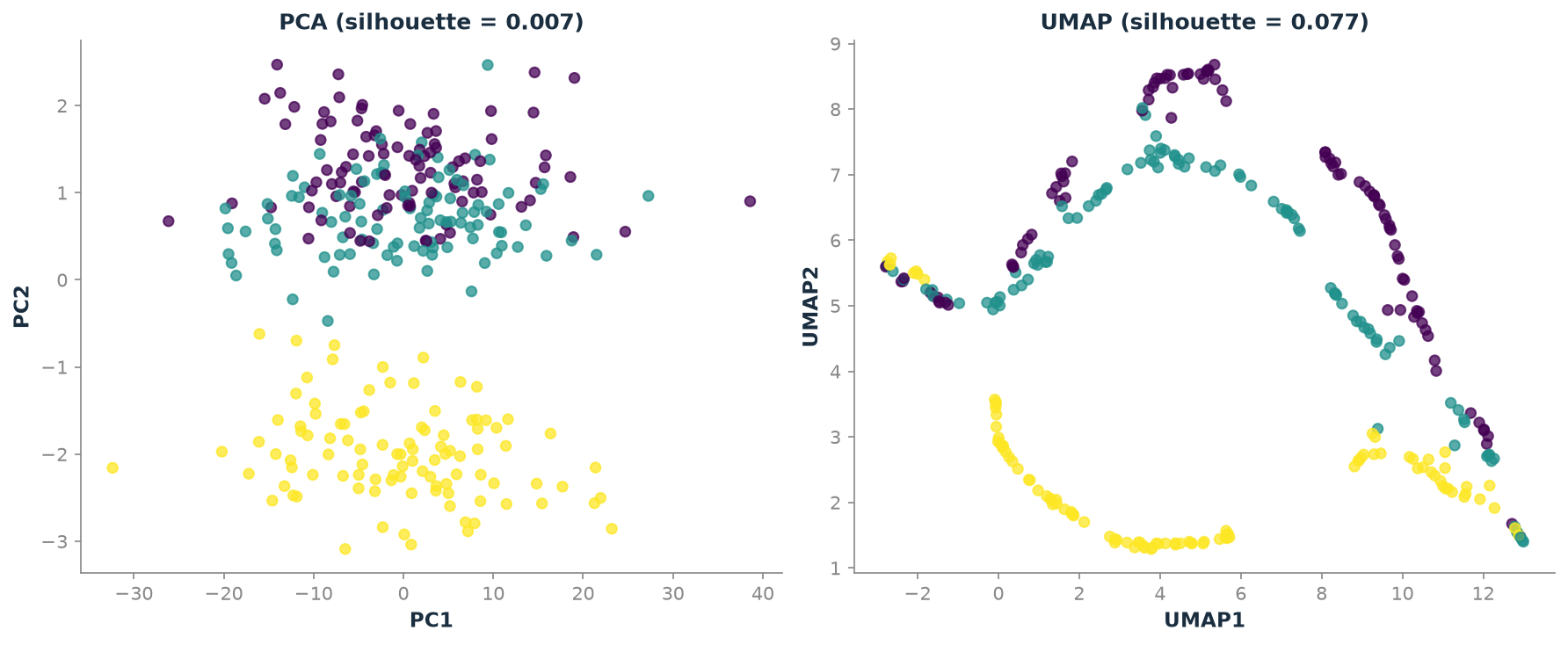
Figure 15.1 is the honest picture, not the idealised one. PCA’s top component chases the noisy nuisance dimension, since it has by far the largest variance. Two of the three clusters (the dark and mid-tone points) merge into a single smeared mass, while the third (the lightest) stays visibly apart. Silhouette score: 0.0073, close to the 0 that means “no cluster structure visible at all.” UMAP does better, but “better” here means partial, not perfect. The lightest cluster separates cleanly, and the dark and mid-tone clusters pull apart along most of their length, though they still touch where the embedding curls back on itself. Silhouette score 0.0774, roughly ten times higher than PCA’s: a real and measured improvement, not a clean sweep.
t-SNE, run on the same data with its default settings, is the surprise: 0.0033, worse than PCA, not better. That’s not a bug in the method. t-SNE builds its neighbourhood graph from distances measured in the original feature space, the same space where the noise dimension’s huge scale already dominates every pairwise distance. A method built to preserve local neighbourhoods still inherits whatever those neighbourhoods look like in the raw data, noise dimension included, unless something else, a smaller perplexity, a prior scaling step, counteracts it. Rerunning with perplexity=12 instead of the default 30 gives 0.107, better than UMAP, on the exact same data. That swing, from worse-than-PCA to better-than-UMAP on one hyperparameter change, is the sensitivity this chapter’s Trade-offs section warns about, made concrete.
The moral isn’t “UMAP is better than PCA,” and it isn’t “t-SNE and UMAP always fix this” either. PCA’s global-variance objective can be actively misled by a single noisy, high-variance column that has nothing to do with the structure that matters. A local-structure method recovers some of what PCA lost, but only if its own settings are tuned to the data, and a default configuration is no guarantee of that. That’s exactly why it’s worth looking at the real picture, with real numbers, instead of assuming the textbook one.
There are three separate reasons their output shouldn’t feed a model, though. First: both are typically non-parametric in their classic form. There’s no simple transform() for new data with the same guarantee as the fitted embedding. UMAP supports transform() with caveats, while classic t-SNE does not, without retraining on the combined dataset. Second: distances between clusters in the embedding aren’t meaningful. Only local neighbourhood structure within a cluster is preserved reliably, so two clusters that look far apart aren’t necessarily “more different” than two that look close. Third: both are stochastic and sensitive to hyperparameters (perplexity for t-SNE; n_neighbors and min_dist for UMAP). Rerunning with a different seed or parameter can meaningfully change the layout. That’s fine for a one-off exploratory plot, but a poor foundation for a reproducible production feature. Use t-SNE and UMAP to look at data: check whether classes separate, spot outlier clusters, sanity-check a clustering result from Chapter 19. Use PCA, or regular feature selection, when reduced dimensions need to feed a model.
15.3 Trade-offs and Limits
Selection preserves interpretability and is safe to defend to a stakeholder (“we use income and tenure”). Extraction squeezes out more redundancy but gives up that interpretability entirely. Filters are cheap and model-agnostic, but ignore feature interactions. Wrappers are thorough, but expensive and specific to whichever model did the searching. Embedded methods are the best per-cost trade-off for most tabular problems, and are the reasonable place to start. Between PCA and t-SNE/UMAP: PCA is linear, deterministic, and approximately reversible. An approximation of the original data can be reconstructed from it, which makes it suitable both for visualisation and as a preprocessing step for a downstream model. t-SNE and UMAP are non-linear and much better for visual cluster discovery, but they’re the wrong tool whenever reduced features need to be deployed and explained.
It’s also worth asking whether this chapter’s machinery is needed at all. Tree-based models (Random Forest, XGBoost, LightGBM) are relatively robust to irrelevant features. They won’t split on features that don’t help. Feature selection matters most for linear models, distance-based models (KNN, K-Means), and any case where training cost or interpretability is a real constraint. It is not a required step before training.
15.4 Procedures
Procedure 15.1 (Drop Low-Variance and Highly Correlated Features). When to use: as a first, cheap pass before any modelling, to remove features that are almost constant or redundant with another feature.
from sklearn.feature_selection import VarianceThreshold
import pandas as pd
import numpy as np

# Drop near-constant columns (threshold is variance, not
# std, tune for your scale)
selector = VarianceThreshold(threshold=0.01)
X_reduced = selector.fit_transform(X_train)
kept_columns = X_train.columns[selector.get_support()]

# Drop one of each highly-correlated pair
corr_matrix = X_train.corr().abs()
upper_mask = np.triu(np.ones(corr_matrix.shape), k=1).astype(bool)
upper = corr_matrix.where(upper_mask)
to_drop = [col for col in upper.columns if any(upper[col] > 0.95)]
X_train_decorrelated = X_train.drop(columns=to_drop)
Common mistake: running VarianceThreshold on unscaled data. A feature ranging 0-1,000,000 will always look “high variance” even if it’s useless, while a feature ranging 0-1 might get dropped even if it’s highly predictive. Scale first, or reserve variance thresholding for features already on comparable scales such as one-hot encoded columns.
Procedure 15.2 (Select Features by Mutual Information). When to use: a fast, non-linear-aware ranking of features against the target, without training a full model.
from functools import partial
from sklearn.feature_selection import (
    mutual_info_classif,
    mutual_info_regression,
    SelectKBest,
)

mi_scores = mutual_info_classif(X_train, y_train, random_state=42)
mi_ranking = (
    pd.Series(mi_scores, index=X_train.columns)
    .sort_values(ascending=False)
)

# mutual_info_classif is randomised: seed it here too
mi_seeded = partial(mutual_info_classif, random_state=42)
selector = SelectKBest(score_func=mi_seeded, k=10)
X_selected = selector.fit_transform(X_train, y_train)
selected_columns = X_train.columns[selector.get_support()]
# For a regression target, use mutual_info_regression instead
Common mistake: computing mutual information, or any selection statistic, on the full dataset before the train/test split: that leaks test-set information into the feature-selection decision. Fit the selector on the training fold only, then apply the same selected columns to the test set.
Procedure 15.3 (Run Recursive Feature Elimination). When to use: finding the feature subset that most helps a specific model, when retraining it repeatedly is affordable.
from sklearn.feature_selection import RFE, RFECV
from sklearn.ensemble import RandomForestClassifier

model = RandomForestClassifier(n_estimators=100, random_state=42)
rfe = RFE(estimator=model, n_features_to_select=10, step=1)
rfe.fit(X_train, y_train)
selected_columns = X_train.columns[rfe.support_]

# Let cross-validation choose the count automatically
# (preferred: avoids guessing)
rfecv = RFECV(estimator=model, step=1, cv=5, scoring='accuracy')
rfecv.fit(X_train, y_train)
print(f"Optimal number of features: {rfecv.n_features_}")
selected_columns = X_train.columns[rfecv.support_]
Common mistake: using a slow model (a deep neural network, a large XGBoost ensemble) inside RFE. Each elimination step retrains from scratch, so runtime multiplies by the number of features removed. Use a fast, well-regularised model for the search; it’s not being deployed, only used to rank features.
Procedure 15.4 (Use Tree-Based Feature Importance for Selection). When to use: a tree ensemble is already in use, or affordable to fit, and selection is wanted essentially for free.
from sklearn.ensemble import RandomForestClassifier
from sklearn.feature_selection import SelectFromModel

rf = RandomForestClassifier(n_estimators=200, random_state=42)
rf.fit(X_train, y_train)

importances = (
    pd.Series(rf.feature_importances_, index=X_train.columns)
    .sort_values(ascending=False)
)

selector = SelectFromModel(rf, prefit=True, threshold='median')
X_selected = selector.transform(X_train)
Common mistake: trusting importance rankings blindly when features are highly correlated. Tree models split arbitrarily between two near-identical correlated features, diluting importance across both and making each look less important than a single, non-redundant version would. Decorrelate first (Procedure 15.1) if this matters.
Procedure 15.5 (Choose the Number of PCA Components). When to use: after deciding PCA is appropriate (linear structure, a need for a reproducible transform) before fitting the final model.
from sklearn.preprocessing import StandardScaler
from sklearn.decomposition import PCA
import matplotlib.pyplot as plt
import numpy as np

# Always scale first
X_scaled = StandardScaler().fit_transform(X_train)

pca_full = PCA().fit(X_scaled)
cumulative_variance = np.cumsum(pca_full.explained_variance_ratio_)

plt.plot(
    range(1, len(cumulative_variance) + 1),
    cumulative_variance,
    marker='o',
)
plt.axhline(
    0.95, color='red', linestyle='--', label='95% variance'
)
plt.xlabel('Number of components')
plt.ylabel('Cumulative explained variance')
plt.legend()
plt.show()

# Or just ask for a variance target directly:
# sklearn picks the count
pca = PCA(n_components=0.95)
X_pca = pca.fit_transform(X_scaled)
print(f"Components needed for 95% variance: {pca.n_components_}")
Common mistake: fitting PCA on training and test data combined “to get a stable transform”: this leaks test-set variance structure into the transform. Fit on training data only, and call .transform(), never .fit_transform(), on the test set.
Procedure 15.6 (Interpret PCA Loadings). When to use: explaining, even approximately, what a principal component “means.”
pca = PCA(n_components=3).fit(X_scaled)

loadings = pd.DataFrame(
    pca.components_.T,
    columns=[f'PC{i+1}' for i in range(3)],
    index=X_train.columns,
)

print(loadings['PC1'].abs().sort_values(ascending=False).head(5))
A large positive or negative loading means that feature strongly drives the component: the sign indicates direction only, not importance. If PC1 loads heavily and positively on income, credit_limit, and spend, it’s roughly “overall financial scale,” but that’s a rough label, not a rigorous claim.
15.5 Worked Example
The tutorial notebook builds a synthetic classification dataset with 50 features: 10 truly informative, 10 redundant (linear combinations of the informative ones), and 30 pure noise. It then runs every selection and extraction technique against it and compares downstream Random Forest accuracy and fit time. A baseline using all 50 features scores:
def evaluate(X_tr, X_te, y_tr, y_te, label, model=None):
    if model is None:
        model = RandomForestClassifier(
            n_estimators=200, random_state=RANDOM_SEED
        )
    start = time.time()
    model.fit(X_tr, y_tr)
    fit_time = time.time() - start
    acc = model.score(X_te, y_te)
    print(
        f"{label:32s} | n_features={X_tr.shape[1]:3d} | "
        f"fit_time={fit_time:.3f}s | test_accuracy={acc:.4f}"
    )
    return {
        "label": label,
        "n_features": X_tr.shape[1],
        "fit_time": fit_time,
        "accuracy": acc,
    }
Running the full comparison on a 1,500-row training split (2,000 samples, 25% held out, random_state=42 throughout) produces:
| Method | Features | Fit time (s) | Test accuracy |
|---|---|---|---|
| Wrapper: RFECV | 26 | 0.552 | 0.928 |
| Embedded: RF importance (median threshold) | 25 | 0.550 | 0.922 |
| Baseline (all 50 features) | 50 | 0.754 | 0.912 |
| Filter: mutual information (top 15) | 15 | 0.397 | 0.884 |
| Extraction: PCA (37 components) | 37 | 0.705 | 0.868 |
The pattern matches what this chapter’s Trade-offs section predicts. RFECV and the embedded Random Forest importance method don’t just match the 50-feature baseline, they beat it, using roughly half the columns and shedding noise features that were otherwise available for the model to overfit on. The mutual-information filter and PCA extraction trail the baseline here, by 2.8 and 4.4 points. PCA’s 37-component result is a reminder. Sometimes real informative structure is spread across many original dimensions, not just redundancy to compress. Then extraction can lose a little relative to a wrapper method that gets to see actual downstream accuracy during selection. Mutual information’s top-15 list: feature_0, feature_5, feature_6, feature_7, feature_9, feature_18, feature_23, feature_25, feature_26, feature_37, feature_38, feature_43, feature_45, feature_48, feature_49. Those names don’t say which features are informative: make_classification shuffles its columns by default. The notebook rebuilds the data with shuffle=False, which puts the informative and redundant features in feature_0 to feature_19, to check the filter against the ground truth.
On the extraction side, fit PCA() with no component limit on the scaled 50-feature training set and read the cumulative explained-variance curve. 37 components are needed to reach 95% of the variance. Not a dramatic compression. After scaling, every column has the same variance, so the 30 pure-noise columns hold about 60% of the total. PCA ranks directions by variance alone, so it can’t skip the noise, and it needs most of those noise directions to reach 95%.
pca_full = PCA(random_state=RANDOM_SEED).fit(X_train_scaled)
cumulative_variance = np.cumsum(pca_full.explained_variance_ratio_)
n_components_95 = np.argmax(cumulative_variance >= 0.95) + 1
print(
    f"Components needed for 95% variance: {n_components_95} "
    "(out of 50 original features)"
)
The second half of the notebook switches from modelling to pure visualisation. It loads the classic 64-pixel handwritten-digits dataset (1,797 samples, 10 classes) and compares PCA, t-SNE, and UMAP as they each compress it to 2D. Timing the three on this machine: PCA runs in 0.05s, t-SNE in 1.54s, and UMAP in 8.58s. PCA’s near-instant linear projection is the expected result. UMAP’s time here is mostly one-off compilation on its first call. On larger datasets, UMAP is usually faster than t-SNE. Visually, plotting each embedding coloured by true digit class, PCA produces a reasonable but often overlapping scatter, since it optimises for global variance rather than class separation. t-SNE and UMAP never see the labels, yet typically produce much tighter, more visually distinct clusters per digit. Both are explicitly preserving local neighbourhood structure rather than total spread.
15.6 AWS SageMaker Notes
# SageMaker's built-in PCA algorithm: useful for very
# large datasets that don't fit in memory on a single
# machine (distributed PCA)
import sagemaker
from sagemaker import PCA as SageMakerPCA

pca_estimator = SageMakerPCA(
    role=role,
    instance_count=1,
    instance_type='ml.m5.xlarge',
    num_components=10,
    mini_batch_size=200,
)
# pca_estimator.fit(train_data_s3_uri)

# For feature selection at scale, SageMaker Data Wrangler
# includes a "Balance and Feature Correlation" analysis
# plus a "Feature Importance" report that combines with
# the same drop-column transforms used above.
When to prefer SageMaker’s built-in PCA: only when the dataset doesn’t fit in memory on one machine. For anything that fits comfortably in a pandas DataFrame, sklearn.decomposition.PCA is simpler and just as correct.
15.7 History and Further Reading
Murphy’s Introduction, Chapter 20, works through the PCA derivation both via eigendecomposition and via SVD with worked examples (Murphy 2022). Burkov gives a concise treatment of dimensionality reduction and feature selection side by side (Burkov 2019, 9). Géron’s Hands-On Machine Learning, Ch. 8, works through PCA and kernel PCA with Scikit-Learn code, a practical complement to this chapter’s derivations and its brief kernel PCA note above. It also covers LLE, a dimensionality-reduction technique not included here (Géron 2019). Wattenberg et al.’s “How to Use t-SNE Effectively” (distill.pub, 2016) is essential reading before trusting any t-SNE plot. The UMAP documentation’s “How UMAP Works” gives an accessible account of the algorithm’s topological motivation. Both are worth reading in full before either technique is used to justify a claim about data structure.
15.8 How This Connects
This chapter builds on Chapter 3’s linear algebra (PCA is an eigendecomposition of the covariance matrix) and on the mutual information machinery from Chapter 5, one of the filter-selection criteria used above. It also assumes Chapter 14’s feature engineering has already produced the candidate columns being pruned here. It enables Chapter 16 (Model Evaluation), since a smaller, cleaner feature set is usually easier to evaluate and less prone to overfitting-driven metric inflation. It also enables Chapter 19 (Unsupervised Learning), where t-SNE/UMAP visualisation is a standard way to sanity-check a clustering result. It’s often confused with feature engineering (Chapter 14): engineering creates candidate features, while this chapter reduces them.
15.9 Exercises
[W] Explain in your own words why feature selection preserves interpretability while feature extraction does not, using the “income is still income” framing from this chapter.
[W] Classify each of the following as a filter, wrapper, or embedded method, and give one reason: (a) dropping features with variance below 0.01; (b) RFECV; (c) keeping features with Random Forest importance above the median.
[A] Using Listing 15.3 as a starting point, rerun mutual-information selection with
k=5instead ofk=10on the synthetic dataset from Listing 15.8, and report whether the resulting 5 features are a subset of the 15 reported in the Worked Example.[A] Using Listing 15.9’s logic, find how many components are needed to reach 99% cumulative explained variance on the same 50-feature training set, and compare the result to the 37 needed for 95%.
[A] Reproduce the digits-dataset PCA vs. t-SNE timing comparison from the Worked Example, but with
perplexity=5instead ofperplexity=30in the t-SNE call. Describe qualitatively how the resulting 2D plot’s cluster tightness changes.[E] The Worked Example shows RFECV and embedded Random Forest importance both beating the 50-feature baseline. Using the curse of dimensionality from this chapter’s Exposition, explain why removing features can improve accuracy rather than merely preserving it.
[E] A regulator requires that a credit-scoring model’s predictions be explainable in terms of the original applicant-provided variables. A colleague proposes using PCA to cut a 200-feature dataset down to 20 components first. Write two or three sentences explaining why this is likely to cause a problem, and what you’d suggest instead.
[R] Read the Wattenberg et al. “How to Use t-SNE Effectively” piece cited above. Identify one t-SNE pitfall it describes that this chapter did not mention, and explain how it would change the interpretation of the digits-dataset t-SNE plot in the Worked Example.
15.10 Mental Model
Feature engineering fills a toolbox. Feature selection and dimensionality reduction decide which tools are needed for the job in front of you. Selection removes tools that won’t be used. Extraction welds several overlapping tools down into one multi-purpose one. Both exist because a toolbox that’s overflowing slows everything down, hurting more than it helps.