Chapter 14
Feature Engineering
Cross-validation is set up correctly. A bunch of algorithms have been tried. Accuracy is stuck. Nothing gets past a mediocre ceiling. The bottleneck isn’t the model. It’s the features. A model can only work with the signal it’s given. Say the information needed to make a good prediction is buried in the raw data, in a form the model can’t see. No amount of algorithmic cleverness closes that gap. This chapter is about making that hidden information visible.
14.1 Motivation
A feature is a measurable property of an observation that a model uses to predict. Feature engineering transforms raw data into features that make patterns easier to learn. The question to ask of every column: what information is latent in this data that the model currently can’t see? A datetime column contains day-of-week, time-of-day, holiday status, and recency, all at once. An address contains a city, a region, a distance to a point of interest. A text description contains sentiment, keywords, length. Feature engineering extracts these hidden signals and presents them explicitly. It doesn’t leave the model to guess at them from a single opaque column.
14.2 Exposition
14.2.1 Numeric Feature Transformations
Scaling matters for linear and distance-based models (KNN, SVM), which are sensitive to feature magnitude. A feature measured in thousands (income) will dominate one measured in single digits (age) unless scaled. StandardScaler (subtract mean, divide by std) is the default choice. MinMaxScaler (scale to ) suits bounded-input needs like neural networks. RobustScaler (median and IQR instead of mean and std) suits data with real outliers. Tree-based models (Random Forest, XGBoost) split on thresholds, not magnitudes. They need no scaling at all.
Log transforms compress the right tail of right-skewed distributions (income, price, population), where a few very large values drag the mean far from the median. np.log1p (which handles zeros safely) gives the model a more balanced signal, and is worth reaching for whenever a histogram of the feature looks like an exponential curve.
import numpy as np
import matplotlib.pyplot as plt

rng = np.random.RandomState(42)
income = rng.lognormal(mean=10.5, sigma=0.6, size=2000)

fig, axes = plt.subplots(1, 2, figsize=(12, 4))

axes[0].hist(income, bins=40, color='#4E79A7')
axes[0].axvline(income.mean(), color='#999999', linestyle='--', label='mean')
axes[0].axvline(np.median(income), color='#4E79A7', linestyle=':',
                linewidth=2.5, label='median')
axes[0].set_title('Raw income: mean pulled right of the median')
axes[0].legend()

log_income = np.log1p(income)
axes[1].hist(log_income, bins=40, color='#59A14F')
axes[1].axvline(log_income.mean(), color='#999999', linestyle='--', label='mean')
axes[1].axvline(np.median(log_income), color='#4E79A7', linestyle=':',
                linewidth=2.5, label='median')
axes[1].set_title('log1p(income): mean and median nearly coincide')
axes[1].legend()
plt.tight_layout()
plt.show()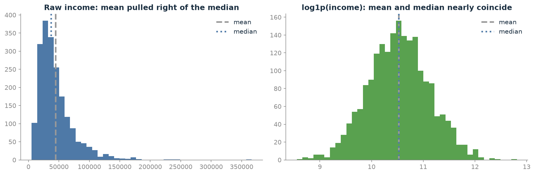
Figure 14.1 shows exactly the pattern the maths predicts. Raw income has mean 44,543 sitting well above median 37,302, the long right tail pulling the average away from where most of the mass is. The log-transformed version has mean 10.5271 against median 10.5268, close enough to call the same number. That’s the visual signature of a distribution the model can now treat as roughly symmetric.
Polynomial features let linear models capture non-linear relationships they otherwise can’t represent. If depends on quadratically (a sweet spot where too little or too much of is bad), adding explicitly via PolynomialFeatures is what lets a linear model see that curvature.
X = rng.uniform(-5, 5, 300)
y = -(X - 1) ** 2 + 10 + rng.normal(0, 1.5, 300)

fig, axes = plt.subplots(1, 2, figsize=(12, 4))

axes[0].scatter(X, y, alpha=0.5, color='#4E79A7')
axes[0].set_xlabel('X')
axes[0].set_ylabel('y')
axes[0].set_title('y vs. X: a straight line can\'t follow this curve')

axes[1].scatter((X - 1) ** 2, y, alpha=0.5, color='#59A14F')
axes[1].set_xlabel('(X-1)²')
axes[1].set_ylabel('y')
axes[1].set_title('y vs. (X-1)²: now a straight line fits')
plt.tight_layout()
plt.show()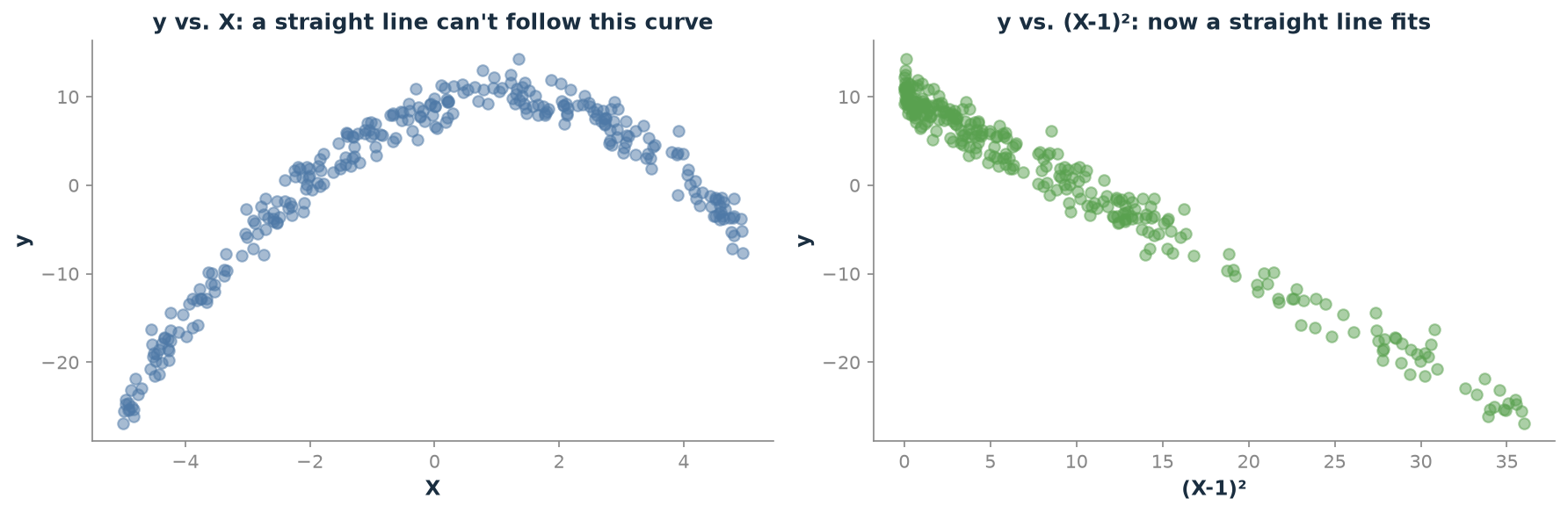
Figure 14.2 is the same curvature a linear model sees when it’s only given . Whatever line it draws, it’s wrong at both ends or wrong in the middle. The correlation between and measures a modest 0.62. The right panel is the identical data, re-expressed on . The curve has been straightened out entirely by the feature, not by the model: correlation jumps to -0.99, close to the -1 of a perfectly linear relationship (negative, since further from the sweet spot at means lower ). That’s the whole point of adding the feature explicitly, rather than hoping a linear model discovers the relationship on its own.
Binning converts a continuous variable into discrete categories, useful when the true relationship is non-linear but step-like (age groups in marketing, income brackets in insurance) via pd.cut or KBinsDiscretizer.
14.2.2 Categorical Feature Encoding
Models need numbers, so categorical variables must be converted. One-hot encoding creates a binary column per category. It’s best for nominal categories (no natural order) with low cardinality (under roughly 20 unique values). Label/ordinal encoding assigns an integer per category. This is only safe when the categories have a genuine order (poor < fair < good < excellent), or when the downstream model is tree-based and won’t be misled by a false ordering. A linear model fed label-encoded nominal categories will treat category 2 as “twice” category 1, an ordering that doesn’t exist. Target encoding replaces each category with the mean of the target for that category. It handles high cardinality (postal codes, product IDs, user IDs) where one-hot would explode into thousands of columns. But it leaks label information if done naively. It must always be computed with fold-holdout cross-validation, never a single global mean. Frequency encoding replaces each category with how often it appears. It never looks at the label, so it carries no label leakage, and captures the idea that rare categories may behave differently from common ones.
14.2.3 Datetime Feature Extraction
A single datetime column hides hour, day-of-week, month, year, weekend/holiday status, and days-since-a-reference-point. All extractable directly via .dt accessors. For cyclical features (hour, day of week, month), the raw integer gets the distance wrong: hour 23 and hour 0 are one hour apart in reality but 23 apart numerically. Cyclical (sin/cos) encoding fixes this by mapping the cycle onto a circle, so adjacent-in-time values stay numerically adjacent.
fig, axes = plt.subplots(1, 2, figsize=(11, 5))

hours = np.arange(24)
axes[0].scatter(hours, np.zeros_like(hours), c=hours, cmap='twilight', s=60)
for h in [0, 6, 12, 18, 23]:
    axes[0].annotate(str(h), (h, 0), textcoords='offset points', xytext=(0, 10))
axes[0].set_yticks([])
axes[0].set_xlabel('raw hour')
axes[0].set_title('Raw hour: 23 and 0 sit at opposite ends')
axes[0].spines['left'].set_visible(False)

hour_frac = 2 * np.pi * hours / 24
hour_sin, hour_cos = np.sin(hour_frac), np.cos(hour_frac)
axes[1].scatter(hour_cos, hour_sin, c=hours, cmap='twilight', s=60)
for h in [0, 6, 12, 18, 23]:
    axes[1].annotate(str(h), (hour_cos[h], hour_sin[h]),
                     textcoords='offset points', xytext=(5, 5))
axes[1].set_xlabel('hour_cos')
axes[1].set_ylabel('hour_sin')
axes[1].set_title('sin/cos hour: 23 sits right next to 0')
axes[1].set_aspect('equal')
plt.tight_layout()
plt.show()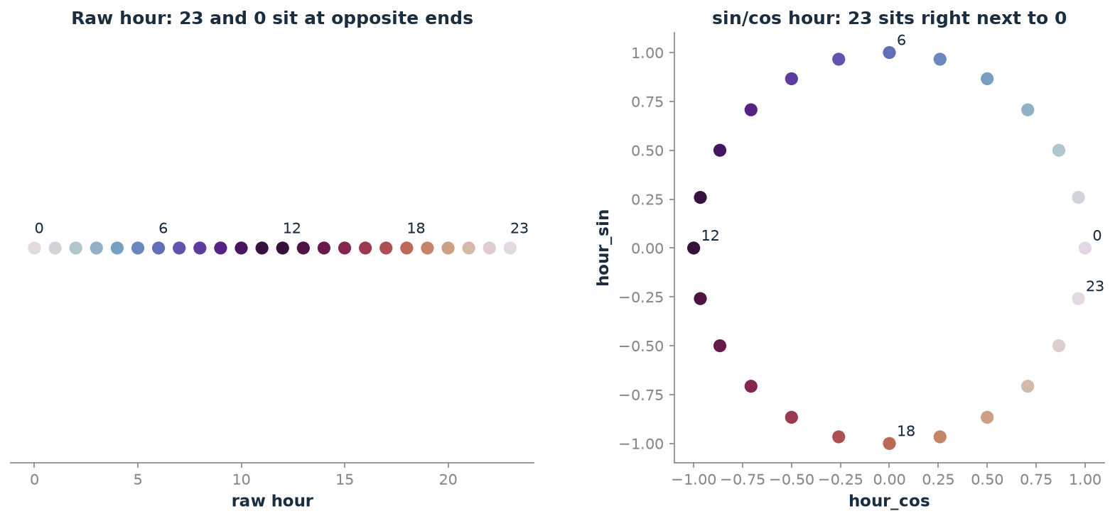
On the left of Figure 14.3, the raw hour axis puts 23 and 0 as far apart as two numbers can be, even though midnight to 11pm is one hour. On the right, the same 24 hours plotted as (hour_cos, hour_sin) coordinates fall on a circle. 23 lands right beside 0, exactly the adjacency the raw integer got wrong.
14.2.4 Interaction Features
An interaction feature is the product or ratio of two features. It captures a joint effect neither captures alone. Square metres and neighbourhood are each important for house price, but their interaction is what matters. A large house in an expensive neighbourhood is worth far more than the sum of a generic “large house” premium and a generic “good neighbourhood” premium. Tree-based models implicitly build interactions through their splits, so explicit interaction features matter less for them. For linear models, they’re often essential to capture non-additive effects at all.
14.2.5 Domain-Specific Features
The highest-leverage features usually come from domain knowledge, not generic transformations. For churn prediction, Recency (days since last purchase), Frequency (purchases in the last 90 days), and Monetary value (RFM, a decades-old direct-marketing framework) often outperform raw transaction data. They capture what drives churn, rather than a generic statistical summary of it. The best feature engineers spend the time talking to domain experts before writing code.
RFM scores every customer on three numbers, each computed straight from transaction history: Recency, days since their last purchase; Frequency, how many purchases they’ve made in a fixed window; and Monetary, how much they’ve spent in that window. The framework predates machine learning by decades. Direct-mail marketers used it by hand, ranking customers into quintiles on each dimension and mailing only to the highest-scoring segments. Postage cost money, and a badly-targeted catalogue was a real loss, not just a wasted API call (Hughes 1994). As three engineered features, RFM works for the same reason it worked on paper: a customer who bought recently, buys often, and spends a lot is a very different prospect from one who did all three once, years ago. Each of the three numbers on its own is a weaker signal than the combination. Recency alone doesn’t distinguish a big spender from a one-off. Frequency alone doesn’t distinguish someone buying small items constantly from someone who checked in twice with two large orders. It’s a domain-knowledge feature in the purest sense. Nothing about the transaction table forces this particular three-number summary to be the useful one. It took decades of direct-marketing practice to establish that it is.
14.3 Trade-offs and Limits
More features raise overfitting risk. Each addition should be validated with cross-validation. Feature engineering is also a leakage risk. Any feature using information from the future, or from the test set, produces optimistic training results that fail in production. Target encoding is the pointiest version of this trap. It’s easy to compute correct-looking statistics on the wrong data. Scaling is part of the preprocessing pipeline, fit on training data only, then applied (never re-fit) to test data.
14.4 Procedures
Procedure 14.1 (Choose Between One-Hot, Ordinal, and Target Encoding). When to use: deciding how to encode any categorical column.
# One-hot: nominal, low cardinality (< ~20)
from sklearn.preprocessing import OneHotEncoder
encoder = OneHotEncoder(
    handle_unknown='ignore', sparse_output=False
)

# Ordinal: genuine order (poor < fair < good < excellent)
from sklearn.preprocessing import OrdinalEncoder
encoder = OrdinalEncoder(
    categories=[['poor', 'fair', 'good', 'excellent']]
)

# Target/mean encoding for high cardinality: ALWAYS via
# CV-encoding, never a single global mean
Common mistake: using integer label encoding for a nominal column feeding a linear model. The model will read category 2 as “twice” category 1.
Procedure 14.2 (Target-Encode Without Leaking the Label). When to use: a high-cardinality categorical where frequency encoding isn’t informative enough.
def cv_target_encode(
    X_train, y_train, X_test, column, n_splits=5, smoothing=10
):
    global_mean = y_train.mean()
    train_encoded = pd.Series(index=X_train.index, dtype=float)
    kf = KFold(n_splits=n_splits, shuffle=True, random_state=42)
    for tr_idx, val_idx in kf.split(X_train):
        fold_train = X_train.iloc[tr_idx]
        fold_y = y_train.iloc[tr_idx]
        stats = fold_y.groupby(fold_train[column]).agg(
            ['mean', 'count']
        )
        smoothed = (
            stats['mean'] * stats['count']
            + global_mean * smoothing
        ) / (stats['count'] + smoothing)
        val_rows = X_train.iloc[val_idx][column]
        train_encoded.iloc[val_idx] = (
            val_rows.map(smoothed).fillna(global_mean).values
        )
    full_stats = y_train.groupby(X_train[column]).agg(
        ['mean', 'count']
    )
    full_smoothed = (
        full_stats['mean'] * full_stats['count']
        + global_mean * smoothing
    ) / (full_stats['count'] + smoothing)
    test_encoded = X_test[column].map(full_smoothed).fillna(
        global_mean
    )
    return train_encoded, test_encoded
Common mistake: computing df.groupby(column)[target].mean() on the full dataset before splitting, then mapping it onto both train and test. This bakes test-set target information into every training row.
Procedure 14.3 (Extract Features from a Datetime Column). When to use: any timestamp column.
def add_datetime_features(df, col):
    df = df.copy()
    df[f'{col}_hour'] = df[col].dt.hour
    df[f'{col}_dow'] = df[col].dt.dayofweek
    is_weekend = df[col].dt.dayofweek.isin([5, 6])
    df[f'{col}_is_weekend'] = is_weekend.astype(int)
    hour_frac = 2 * np.pi * df[f'{col}_hour'] / 24
    df[f'{col}_hour_sin'] = np.sin(hour_frac)
    df[f'{col}_hour_cos'] = np.cos(hour_frac)
    return df
Procedure 14.4 (Build a Leakage-Safe ColumnTransformer Pipeline). When to use: a mix of numeric and categorical columns that need to be cross-validated safely as one unit.
numeric_pipe = Pipeline([
    ('impute', SimpleImputer(strategy='median')),
    ('scale', StandardScaler()),
])
categorical_pipe = Pipeline([
    ('impute', SimpleImputer(strategy='most_frequent')),
    ('onehot', OneHotEncoder(handle_unknown='ignore')),
])
preprocessor = ColumnTransformer(transformers=[
    ('num', numeric_pipe, numeric_features),
    ('cat', categorical_pipe, categorical_features),
])
full_pipeline = Pipeline([
    ('preprocess', preprocessor),
    ('model', your_model),
])
Common mistake: calling scaler.fit_transform(X) on the whole dataset before train_test_split. Split first, .fit() on train only, .transform() (never .fit_transform()) on test.
14.5 Worked Example
A synthetic e-commerce order dataset (4,000 orders; features include customer ID, region, payment method, age, items in cart, and an order timestamp; 3,200/800 train/test split) makes the leakage question concrete rather than abstract. Encode the high-cardinality customer_id column two ways: a naive global mean computed across the whole dataset before splitting, versus Procedure 14.2’s fold-holdout CV encoding. Then compare cross-validated on the training set alone:
scores_leaky = cross_val_score(
    ridge, X_train_leaky[feat_cols], y_train, cv=5, scoring='r2'
)
scores_safe = cross_val_score(
    ridge, X_train_safe[feat_cols], y_train, cv=5, scoring='r2'
)
Measured: leaky encoding reports CV . Safe encoding reports . Leaky encoding looks very slightly better, exactly the direction the leakage warning predicts, even though the gap here is modest. Checking the true held-out test for both confirms the honest picture: leaky encoding scores 0.870 on test, safe encoding scores 0.867, nearly identical to their respective CV numbers. Why so close? In this particular synthetic dataset, customer_id isn’t a strongly predictive column on its own. Order value is driven mostly by region, items in cart, and weekend timing, not by which customer placed the order. The lesson this measurement teaches is more precise than “leakage always inflates your score dramatically.” Leakage’s damage scales with how much the leaking column correlates with the target once leaked. A weakly-predictive ID column leaks only a little. A strongly-predictive one (e.g. a column that indirectly encodes the label) can produce the dramatic, disqualifying gap the warnings describe. Measuring the gap, rather than assuming its size, is the only way to know which situation is in play.
The full pipeline (cyclical datetime features, one-hot encoded region and payment method, no customer ID at all) reaches CV and true test . That’s identical to the safely-encoded variant above, and only a hair behind the leaky one. That tie is the real finding. Honestly encoding customer_id costs nothing next to dropping it outright, because the column carries no signal a fold-holdout encoding can safely pull out. The leaky version’s tiny edge comes entirely from peeking at the label, not from customer_id actually mattering.
# SageMaker Data Wrangler: no-code equivalent for scaling,
# encoding, and datetime extraction via a visual flow,
# exportable as a Processing job.

import sagemaker
from sagemaker.feature_store.feature_group import FeatureGroup

feature_group = FeatureGroup(
    name='orders-features',
    sagemaker_session=sagemaker.Session(),
)
# feature_group.create(
#     s3_uri='s3://my-bucket/feature-store/orders/',
#     record_identifier_name='order_id',
#     event_time_feature_name='event_time',
#     role_arn=role, enable_online_store=True)
When to prefer SageMaker Feature Store: when the same engineered feature (e.g. a customer’s frequency encoding) needs to be computed once and served consistently to both a training job and a real-time inference endpoint, preventing training/serving skew.
14.6 History and Further Reading
Thakur, Ch. 4 and 5, cover categorical encoding and feature engineering for various data types with code (Thakur 2020). Murphy’s Introduction, Ch. 9, gives the formal treatment of linear models and feature maps (Murphy 2022). Zheng and Casari’s Feature Engineering for Machine Learning is a full book on the topic (Zheng and Casari 2018).
14.7 How This Connects
This chapter builds on Chapter 7 (clean data before engineering features) and Chapter 9 (EDA is usually where the need for a given transformation is discovered). It enables Chapter 15’s feature selection, which needs features to exist before choosing among them. It also enables Chapter 16’s model evaluation, which is what any feature engineering decision gets judged against in the end. It’s often confused with feature selection: engineering creates new features, while selection chooses which existing features to keep.
14.8 Exercises
[W] Explain why tree-based models don’t need feature scaling while linear and distance-based models do, using the “splits on thresholds, not magnitudes” framing from this chapter.
[W] For each, name the correct encoding from this chapter: (a) a
sizecolumn with valuessmall/medium/large; (b) aproduct_skucolumn with 50,000 unique values feeding a linear model; (c) acountrycolumn with 15 unique values, no natural order.[A] Using Listing 14.6, compute
hour_sin/hour_cosfor hour 23 and hour 0 by hand, and show numerically that their Euclidean distance is small, in contrast to the raw hour values, which differ by 23.[A] Using Listing 14.8’s pattern, explain what result you would expect if
customer_idwere replaced with a column that directly encoded a noisy version of the label (e.g.last_order_value_rounded), would the leaky-vs-safe CV gap this chapter measured (0.872 vs. 0.870) likely grow, shrink, or stay about the same?[E] A teammate wants to one-hot encode a
product_idcolumn with 8,000 unique values “to keep things simple.” Using this chapter’s cardinality guidance, write the two or three sentences you’d say instead.[E] This chapter’s measured leaky-vs-safe gap was small (0.872 vs. 0.870). Using the Worked Example’s explanation for why, describe a realistic feature (not
customer_id) in the same order dataset that would very likely produce a much larger leakage gap if encoded naively.[R] Read the scikit-learn
TargetEncoderdocumentation (orcategory_encoders.TargetEncoder). Identify one detail of its built-in cross-fitting behaviour that differs from Procedure 14.2’s hand-written version, and explain what problem that difference solves.
14.9 Mental Model
Features are the vocabulary a model uses to describe an observation. The richer and more precise that vocabulary, the better the model can describe the pattern it’s trying to learn. Feature engineering is translation work. Taking data in one language (raw measurements) and translating it into the language the model speaks. The numbers that carry signal.