Chapter 16
Model Evaluation
Once a model is trained, a simple question follows: is it good? The naive answer (“measure accuracy”) is almost the wrong one. Choosing the wrong metric means optimising for the wrong thing and shipping a model that fails in production in ways that are surprising to whoever picked the metric. This chapter is about learning to ask “good for what?” before measuring anything.
16.1 Motivation
Every evaluation metric is a choice about what to care about. A fraud-detection model that labels every transaction “not fraud” scores roughly 99.9% accuracy on a typical fraud dataset, because fraud is rare. That model is useless. It catches zero fraud while looking nearly perfect. The metric didn’t lie. Well, not exactly. It answered a question nobody asked. The foundation of all classification evaluation is the confusion matrix: a table that counts what a model got right and wrong, broken down by type. Every metric that follows is a formula built on top of that matrix.
16.2 Exposition
16.2.1 The Confusion Matrix
| Predicted Positive | Predicted Negative | |
|---|---|---|
| Actual positive | True Positive (TP) | False Negative (FN) |
| Actual negative | False Positive (FP) | True Negative (TN) |
A false positive is a “false alarm” (Type I error). A false negative is a “missed it” (Type II error). Which one costs more depends entirely on domain. In cancer screening, missing a cancer (FN) is catastrophic. In spam filtering, flagging a legitimate email (FP) is merely annoying. No metric decision makes sense before that cost asymmetry is written down and understood.
16.2.2 Classification Metrics
Accuracy () is useful only when classes are balanced and both error types cost the same. That combination is rare in practice. Precision () answers “of everything predicted positive, how many were.” It matters when false positives are costly. Recall () answers “of everything actually positive, how many were caught.” It matters when false negatives are costly. F1 (the harmonic mean of precision and recall) gives a single balanced number when both matter and classes are imbalanced. ROC-AUC (Area Under the Receiver Operating Characteristic Curve) measures ranking quality across every possible decision threshold at once (1.0 perfect, 0.5 random). It’s useful for comparing models before a threshold is chosen. PR-AUC (Area Under the Precision-Recall Curve) does the same, but focuses on the positive class specifically. It’s the more honest choice under heavy imbalance, where ROC-AUC can look deceptively good. Log loss penalises confident wrong predictions heavily. It matters when the actual probability, not just the ranking, is going to drive a decision.
The familiar mean, , treats a strong score and a weak one as interchangeable. Precision 1.0 and recall 0.01 average out to 0.505, which reads as “roughly middling” for a model that in practice catches almost nothing. The harmonic mean, , doesn’t average the two numbers so much as average their reciprocals. That pulls the result sharply towards whichever number is smaller. The same precision 1.0 and recall 0.01 give a harmonic mean of 0.0198, close to the useless 0.01 and nothing like the reassuring 0.505 the arithmetic mean reported. That’s exactly the property F1 needs. A model has to do reasonably well on both precision and recall to get a good F1 score. A harmonic mean can’t be dragged up by one strong number covering for one weak one the way an arithmetic mean can.
16.2.3 The Precision-Recall Trade-off
A classifier outputs a probability, not a label. A threshold (commonly 0.5) turns that probability into a decision. Lowering the threshold predicts positive more often, raising recall at the cost of precision. Raising the threshold does the opposite. There is no free lunch. The PR curve shows every trade-off point at once. The business context, what an FP costs versus what an FN costs, is what tells you where on that curve to operate.
16.2.4 Regression Metrics
MSE () penalises large errors quadratically and is differentiable, which is why it’s used during training. RMSE () is the same information in the target’s own units. MAE () is less sensitive to outliers than RMSE. A large RMSE/MAE ratio, rule of thumb: above roughly 2x, is a diagnostic that outliers are present and influencing RMSE disproportionately. MAPE gives scale-invariant percentage error but breaks when the target can be zero. gives the proportion of variance: 1 is perfect, 0 means no better than predicting the mean, and negative means actively worse than that trivial baseline.
16.2.5 Calibration
Calibration asks a simple question: when a model says 70% probability, is it right 70% of the time? A model can separate positives from negatives well, good discrimination, e.g. high ROC-AUC, while still being poorly calibrated. Its probabilities are systematically over- or under-confident. Calibration matters when the probability itself drives a decision. Insurance pricing, medical risk scores, and financial models all need calibrated probabilities, not just correctly-ordered ones. The reliability diagram plots predicted-probability bins against observed frequency. A perfectly calibrated model lies on the diagonal. Random Forests are a common source of S-shaped miscalibration. Their probabilities rarely reach 0 or 1, so they are under-confident at the extremes. Naive Bayes shows the opposite pattern: over-confident. Fixable with isotonic regression or Platt scaling via CalibratedClassifierCV.
16.2.6 The Business Metric Gap
An ML metric and a business metric are different things. Minimising RMSE on a demand forecast doesn’t maximise profit, because the costs of over-stocking and under-stocking are rarely symmetric. The right question is “what does a unit improvement in this ML metric get us in business terms.” Not “is this ML metric improving.”
16.3 Trade-offs and Limits
Accuracy is acceptable with balanced classes, symmetric error costs, and a rough model-to-model comparison in mind. It misleads under class imbalance: prefer F1 or PR-AUC there. It misleads when error costs differ: choose precision or recall based on which error is expensive. And it misleads whenever probabilistic output itself matters: prefer log loss plus calibration checking there instead.
16.4 Procedures
Procedure 16.1 (Compute All Classification Metrics at Once). When to use: immediately after getting predictions from any classifier.
from sklearn.metrics import classification_report, confusion_matrix

y_pred = model.predict(X_test)
y_proba = model.predict_proba(X_test)[:, 1]

print(classification_report(y_test, y_pred))
cm = confusion_matrix(y_test, y_pred)
Procedure 16.2 (Plot the ROC and Precision-Recall Curves). When to use: comparing models’ discrimination ability, or picking a threshold.
import matplotlib.pyplot as plt
from sklearn.metrics import (
    roc_curve,
    roc_auc_score,
    precision_recall_curve,
    average_precision_score,
)

fig, axes = plt.subplots(1, 2, figsize=(12, 5))

fpr, tpr, _ = roc_curve(y_test, y_proba)
auc = roc_auc_score(y_test, y_proba)
axes[0].plot(fpr, tpr, color='#4E79A7',
             label=f'Logistic Regression (AUC = {auc:.3f})')
axes[0].plot(
    [0, 1], [0, 1], color='#999999', linestyle='--', linewidth=1.5,
    label='Random classifier (AUC = 0.5)',
)
axes[0].set_xlabel('False Positive Rate')
axes[0].set_ylabel('True Positive Rate (Recall)')
axes[0].set_title('ROC Curve')
axes[0].legend()

precision, recall, _ = precision_recall_curve(y_test, y_proba)
ap = average_precision_score(y_test, y_proba)
axes[1].plot(recall, precision, color='#E15759',
             label=f'Logistic Regression (AP = {ap:.3f})')
axes[1].axhline(
    y_test.mean(), color='#999999', linestyle='--', linewidth=1.5,
    label=f'No-skill baseline ({y_test.mean():.2f})',
)
axes[1].set_xlabel('Recall')
axes[1].set_ylabel('Precision')
axes[1].set_title('Precision-Recall Curve')
axes[1].legend()

plt.tight_layout()
plt.show()
Procedure 16.3 (Adjust the Decision Threshold). When to use: when FP and FN costs differ, or the default 0.5 threshold isn’t optimal.
import numpy as np
from sklearn.metrics import precision_recall_curve

precision, recall, thresholds = precision_recall_curve(
    y_test, y_proba
)
f1_scores = 2 * precision * recall / (precision + recall + 1e-8)
best_threshold = thresholds[np.argmax(f1_scores[:-1])]
Procedure 16.4 (Compute and Fix a Calibration Curve). When to use: when predicted probabilities drive a decision directly.
from sklearn.calibration import (
    calibration_curve,
    CalibratedClassifierCV,
)

prob_true, prob_pred = calibration_curve(
    y_test, y_proba, n_bins=10
)

calibrated = CalibratedClassifierCV(
    model, method='isotonic', cv=5
)
calibrated.fit(X_train, y_train)
Common mistake: trusting a raw model’s predict_proba output as a real probability without checking calibration first. Random Forests, for example, are often under-confident at the extremes.
16.5 Worked Example
On the Breast Cancer Wisconsin dataset (569 examples; logistic regression on standardised features, 80/20 stratified split), the confusion matrix on the 114-example test set comes out as:
cm = confusion_matrix(y_test, y_pred)
# [[41  1]
#  [ 1 71]]
TN=41, FP=1, FN=1, TP=71. That gives accuracy 0.9825, precision 0.9861, recall 0.9861, F1 0.9861, ROC-AUC 0.9954, PR-AUC 0.9971, and log loss 0.0777. On this dataset, roughly balanced (37%/63%) and well-separated by the available features, accuracy and F1 tell essentially the same story. That’s the signal that accuracy is acceptable here specifically because the imbalance is mild and both error types are similarly rare. Running Procedure 16.2 against this same model and test set produces Figure 16.1.
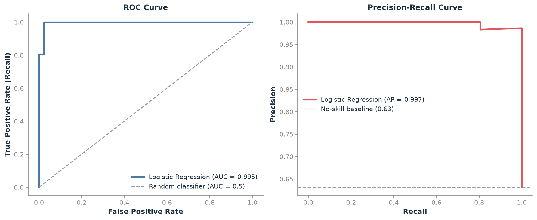
Both curves stay close to their perfect corner for almost their entire length. The ROC curve hugs the top-left. The PR curve stays near precision 1.0 until the last handful of points, where the model’s two mistakes show up as a sharp drop rather than a gradual slide. That’s the visual signature of a model that is right almost everywhere and wrong on only a couple of hard cases.
Sweeping the decision threshold to maximise F1, rather than using the default 0.5, finds a best threshold of 0.366. F1 rises slightly, from 0.9861 to 0.9931: a small but real improvement, and a reminder that even on an easy, well-separated dataset, the default threshold isn’t automatically optimal.
Contrast this with a hypothetical, deliberately harder case: a fraud dataset where only 0.1% of transactions are fraudulent. A model that predicts “not fraud” every time scores accuracy, literally 99.9% correct, while catching exactly zero fraud (recall , precision undefined since ). This isn’t a contrived edge case. It’s the direct arithmetic consequence of accuracy rewarding the majority class, regardless of what the minority class needed the model to do. The breast-cancer dataset’s near-balanced classes are exactly why accuracy behaved reasonably there, and exactly why the same metric would be a lie on a heavily imbalanced problem.
from sagemaker.model_monitor import ModelQualityMonitor

monitor = ModelQualityMonitor(
    role=role, instance_count=1, instance_type="ml.m5.xlarge"
)
monitor.suggest_baseline(
    baseline_dataset=(
        "s3://my-bucket/validation-with-predictions.csv"
    ),
    dataset_format=DatasetFormat.csv(header=True),
    output_s3_uri="s3://my-bucket/baseline/",
    problem_type="BinaryClassification",
    inference_attribute="prediction",
    probability_attribute="probability",
)
monitor.create_monitoring_schedule(
    endpoint_input=endpoint_name,
    schedule_cron_expression="cron(0 * ? * * *)",
)
When to prefer SageMaker Model Monitor: when the metric needs to be tracked continuously against live production traffic, not just computed once on a static test set. It flags metric degradation (e.g. a drop in precision) automatically as the input distribution drifts, rather than waiting for someone to notice.
16.6 History and Further Reading
Thakur, Ch. 6, gives practical metric selection with code examples (Thakur 2020). Géron’s Hands-On Machine Learning, Ch. 3, works through the confusion matrix, precision, recall, and ROC curves on a single running example, a good practical companion to this chapter’s metrics (Géron 2019). Murphy’s Introduction, Ch. 5, gives the formal statistical treatment of evaluation (Murphy 2022). Davis and Goadrich’s paper on the relationship between precision-recall and ROC curves explains why PR-AUC matters specifically under imbalance (Davis and Goadrich 2006).
16.7 How This Connects
This chapter builds on Chapter 11 (a model is needed before it can be evaluated) and on Chapter 13’s cross-validation, since proper evaluation requires the right split strategy applied consistently. It’s often confused with the loss function used during training. The loss is what’s minimised while fitting (often cross-entropy). The evaluation metric is what’s measured afterwards (often F1 or a business-specific number). They are usually different things, measuring related but distinct properties of the same model.
16.8 Exercises
[W] Using the confusion matrix definitions, explain in one sentence each what a false positive and a false negative mean for a spam filter, and state which one is more costly there.
[W] State which metric (precision, recall, or F1) is most appropriate for: (a) a disease-screening test; (b) a spam filter; (c) a general-purpose classifier comparison with no stated cost asymmetry.
[A] Using Listing 16.5, compute precision and recall by hand from TN=41, FP=1, FN=1, TP=71, and confirm they match the reported 0.9861 figures.
[A] Using this chapter’s hypothetical 0.1%-fraud scenario, compute the accuracy of a model that predicts “fraud” for every transaction instead (the opposite extreme), and state its precision and recall.
[E] A customer reports “our fraud model has 99.9% accuracy” as evidence it’s ready to ship. Using this chapter’s Worked Example, write the two or three sentences you’d say before agreeing.
[E] A Random Forest’s
predict_probaoutput is being used directly to set insurance premiums. Using this chapter’s Calibration section, explain what could go wrong and what you’d check before trusting those numbers.[R] Read the Davis and Goadrich (2006) paper’s abstract. Identify the specific claim it makes about ROC curves under class imbalance, and explain how it relates to this chapter’s PR-AUC recommendation for rare-event detection.
16.9 Mental Model
The confusion matrix is the ground truth. Every metric is just a different question asked of that table. Before choosing one, write down what a false positive and a false negative cost in the specific business context. The right metric usually becomes obvious once those costs are made visible.