Chapter 7
Data Cleaning & Wrangling
Real-world data does not arrive clean. It comes from databases with NULLs. Scrapers with encoding errors. Manual entry with typos. Merges with duplicate records. Legacy systems whose type conventions made sense years ago but not today. A model trained on top of that doesn’t average the noise away. It often learns the noise better than the signal. Noise tends to be more systematic than it looks. Every data quality problem reduces to one of a small number of categories, no matter how varied the symptom: missing values, outliers, duplicates, wrong types, encoding errors, inconsistent categories, and schema violations. This chapter builds the diagnostic habit and the treatment toolkit for all seven. It argues that cleaning is not a chore that comes before the real work of data science. For most practitioners, on most projects, it is the real work.
7.1 Motivation
Surveys of data scientists put data preparation and cleaning at anywhere from about 40% to 80% of their working time. Not because they’re inefficient. The work is that large relative to modelling. The reason cleaning matters as much as it does is uneven risk. A model can survive a slightly suboptimal hyperparameter. It cannot survive training on systematically corrupted labels or features. It will faithfully learn the corruption. The discipline this chapter teaches is a repeatable loop that works on any new dataset, regardless of domain, shown in Figure 7.1.
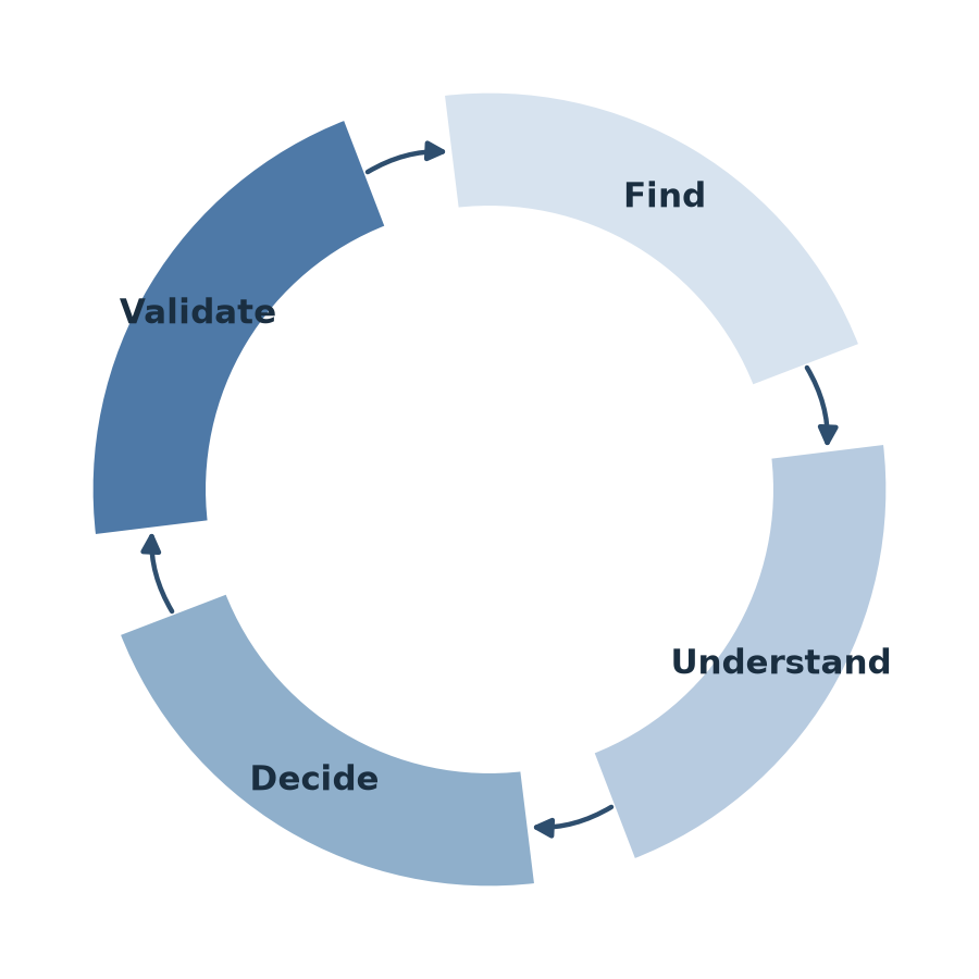
That loop is not unique to data cleaning. It is a special case of an older idea: Boyd’s OODA loop, observe, orient, decide, act. Find is observation: what is in the data. Understand is orientation: why it is there, what produced it. Decide keeps its name. Validate plays the role of act. It checks that the decision, once taken, worked, before the next problem gets the same treatment. Skipping straight to treatment without understanding why a value is missing or unusual is the most common way cleaning goes wrong. It is exactly the failure OODA warns against: acting on an assumption instead of on what the data actually shows.
John Boyd developed the OODA loop as a US Air Force fighter pilot and military strategist, drawing on his analysis of why American F-86 pilots consistently beat the technically superior MiG-15 in Korean War dogfights. His conclusion: the pilot who cycles through observing, orienting, deciding, and acting fastest wins, regardless of whose aircraft is better. Boyd never published the idea as a single paper. It spread through a long unpublished briefing, “Patterns of Conflict,” that he gave throughout the 1970s and 80s. Business strategy, cybersecurity incident response, and sports coaching have since borrowed the loop far outside its military origin, the same way this chapter borrows it for data cleaning.
7.2 Exposition
7.2.1 Missing Values
Missing data is one of three different problems, depending on the mechanism that produced the gap. The mechanism determines which treatments are safe:
- MCAR (Missing Completely At Random): the probability of a value being missing has nothing to do with any other variable: a sensor randomly dropped a reading. This is the safest case: dropping or imputing introduces no systematic bias.
- MAR (Missing At Random): missingness depends on observed variables, not on the missing value itself. Men might be less likely to report their age. But among men, the missing ages aren’t systematically different from the reported ones. This can still be safely imputed, provided the imputation model has access to the variables that predict missingness.
- MNAR (Missing Not At Random): missingness depends on the missing value itself: high earners decline to report income more often than everyone else. This is the dangerous case: naive imputation will systematically underestimate the very quantity being estimated. The mechanism that hides values correlates with those values. MNAR requires explicitly modelling the missingness process, not just filling gaps.
Given a mechanism, imputation strategies form a rough ladder of increasing complexity and (usually) increasing accuracy:
- Drop rows or columns outright.
- Constant fill: a fixed value such as 0,
"Unknown", or a sentinel. - Statistical fill: the column’s own mean, median, or mode (told you mode had a use).
- Forward/backward fill: for time series, where the adjacent value is a reasonable estimate.
- K-nearest-neighbours imputation: estimates a missing value from the most similar rows on other features.
- Model-based imputation: trains a regression or classifier to predict the missing column from the rest.
Climbing the ladder costs complexity and compute, and gets us robustness. Dropping is free but throws away information. KNN and model-based imputation are expensive but respect the structure between features.
7.2.2 Outliers
An outlier is a value far from the rest of a distribution. But “far” is not automatically “wrong.” A CEO’s salary in a company-wide compensation dataset is a real outlier. Treating it as noise discards signal. The question is always: is this outlier informative or harmful?
Two detection methods dominate practice. The IQR (interquartile range) method flags anything outside
and is robust to skew because it’s defined by rank statistics, not the mean.
A rank statistic is computed from the sorted position of values, their rank, rather than their raw magnitude. and are examples: is the value 25% of the way through the sorted data, is the value 75% of the way through, and neither cares how far apart the surrounding values are. Move the largest value in a column from 100 to 100,000 and the mean shifts with it. and don’t move at all, because their position in the sorted order hasn’t changed. That’s the same property Chapter 3 uses to call the median robust to outliers, applied here to quartiles instead of the midpoint.
The z-score method flags any value with
Here is the number of standard deviations sits from the mean , using the mean and standard deviation from Chapter 3. Unlike a rank statistic, is computed from raw magnitude. That’s exactly why it’s simple and interpretable. But it assumes an approximately normal distribution. It’s also somewhat circular: a genuine outlier inflates and can mask itself. Both are single-variable methods. Multivariate anomaly detection (Isolation Forest and its relatives, covered in Chapter 19) is needed when “unusual” only shows up in the combination of features rather than any one alone.
Once detected, treatment is a judgement call:
- Remove a value only when it’s clearly an error, an age of 300, for instance.
- Cap (winsorise) it: replace values beyond a percentile threshold with the threshold. Use this when the value is real but shouldn’t be allowed to dominate a model fit on scale-sensitive algorithms.
- Transform (typically log) a skewed distribution, to compress its tail rather than discard information from it.
- Flag and keep: add a binary
is_outliercolumn and let the model decide. This works well for tree-based models that can split on the flag directly.
7.2.3 Duplicates
Duplicate rows are quietly catastrophic for machine learning. They corrupt evaluation, not just training. If some fraction of the training set is duplicated into the test set, reported accuracy is inflated by testing on examples the model has effectively memorised. The model looks better than it is. That gap only surfaces in production. The check is one line: df.duplicated().sum(). The fix requires judgement. Are the duplicates exact, every column matching? Then dropping is safe. Are they partial, same ID but a different timestamp (a re-submission or an update)? Then the right row to keep, first, last, or the one with the most complete data, depends on what the ID represents.
The same failure mode shows up at a much larger scale with generative AI. Internet-scale pretraining corpora overlap heavily with the questions people later ask these models. A language model’s strong performance on a question is partly recall of material it has already seen, not proof of general reasoning. Performance measurably drops on questions that fall outside that training distribution. Book 2, Chapter 29 covers how transformer models are trained on corpora at this scale, and revisits this memorisation question directly.
7.2.4 Type Coercion
pandas infers each column’s type from its values. One stray entry, such as 'unknown' in a number column, makes the whole column load as text. Dates load as text unless pandas is told to parse them. Operating on such a column as text instead of numbers is a quiet, persistent source of bugs: string comparison orders lexically, so '10' > '9' evaluates to False (because '1' < '9' character-by-character). The numeric comparison 10 > 9 is True. The fix is to validate types immediately after loading data, before any filtering or aggregation touches it. Type errors compound: a wrong-typed column silently produces wrong-typed derived columns.
7.2.5 Encoding Errors
Text has to be stored as bytes. Turning bytes back into characters means picking a character encoding: UTF-8, Latin-1 (ISO-8859-1), Windows-1252, and a handful of others are all still common. Read a file with the wrong one and the bytes don’t change, but the characters they turn back into do. A city name saved as UTF-8 and mistakenly read back as Latin-1 turns São Paulo into São Paulo: the same underlying bytes, decoded through the wrong lookup table. This kind of corruption, known as mojibake, is silent. Nothing crashes. The column still loads, still looks like a string, and one real category quietly splits into two, São Paulo and São Paulo sitting side by side as if they were different cities.
Plain ASCII text (letters, digits, common punctuation) survives a wrong-encoding read unharmed. That’s exactly why encoding errors are easy to miss: they only show up on the accented or non-Latin characters a dataset happens to contain. A column of English-only names can hide the same bug a column of international city names exposes immediately. Detection is mostly a matter of looking: scan value_counts() for a suspicious repeated pattern like à followed by another character, or count non-ASCII bytes directly. The fix, when the corruption follows the common UTF-8-read-as-Latin-1 pattern, is to run the mismatch backwards: re-encode the mangled string as Latin-1 to recover the original bytes, then decode those bytes as UTF-8 to get the real text back. When that round trip doesn’t fully explain the corruption, re-reading the source file with the correct encoding= argument from the start is the safer fix.
7.2.6 Inconsistent Categories
Free-text categorical data is almost always inconsistent. It was typed by different people, systems, or eras. A gender column might contain 'female', 'Female', 'F', 'woman', and 'FEMALE': five spellings of the same underlying category. But to any model that one-hot encodes or otherwise treats string values literally, they’re five distinct categories. The fix is aggressive normalisation: strip whitespace and lowercase as a floor, then explicitly map every observed variant to a small set of canonical values. And check what’s left unmapped. An unmapped value silently becomes missing.
7.2.7 Schema Violations
A schema violation is a value that has the right type but breaks the rule that type is supposed to follow. 'not a date' in a date column is not a type error. Python is perfectly happy holding it as a string. It’s a schema violation: the column’s whole reason for existing is to hold valid dates, and this value doesn’t. The same pattern shows up as a negative age, a percentage over 100, an email address with no @, or a customer ID that points to a customer who was never created. Each of those parses fine and fails silently at the level that matters: meaning, not type.
Type Coercion (above) and schema violations often get caught by the same code, since forcing a column through pd.to_datetime() or pd.to_numeric() with errors='coerce' turns anything that isn’t a date, or isn’t a number, into a missing value automatically. But the two problems aren’t the same thing. Type coercion asks can this be parsed as the right type at all. A schema violation can pass that test and still be wrong: age -5 parses as a perfectly good integer. Catching that kind needs an explicit rule about what the field is allowed to mean, not just what it’s allowed to look like. That’s exactly what Procedure 7.6’s validation rules are for.
7.3 Trade-offs and Limits
The decision of whether to drop or impute a column comes down to how much is missing and why: dropping rows is safe when missingness is under roughly 5% and MCAR. The information loss is small and the bias risk is near zero. Above that threshold, or when the missing column matters to the outcome, imputation preserves far more of the dataset at the cost of introducing an estimate where a real value should be. One rule with no exceptions: never impute the target variable (the label). Doing so is label fabrication. The model would be trained, in part, on predictions of itself.
The decision of whether to remove or cap an outlier follows similar logic. Remove only when the value is clearly an error. Cap when it might be genuine but shouldn’t be allowed to dominate a distance- or gradient-sensitive model. Flag and keep when outliers are themselves predictive. In fraud, sensor-failure, and financial contexts, they often are. The one step in this whole chapter that is never optional is validation. After any cleaning operation, compare the before/after distribution of every column that was touched. A cleaning step that silently collapses meaningful variation (over-aggressive winsorising that flattens a bimodal distribution, for instance) produces a dataset that is cleaner-looking but worse than the original. The damage is now invisible.
7.4 Procedures
Procedure 7.1 (Find and Remove Duplicates). When to use: as the first cleaning step on any new dataset, before anything else touches it.
# How many exact duplicates?
df.duplicated().sum()

# Remove duplicates (keep first occurrence)
df = df.drop_duplicates()
df = df.reset_index(drop=True)

# Deduplicate on a subset of columns
# (e.g. same ID, different timestamps)
df = df.drop_duplicates(subset=['id'], keep='last')
Common mistake: dropping duplicates without reset_index(drop=True) afterwards. The index still has gaps from the removed rows. Later .loc[] lookups that assume labels run from 0 to n−1 then miss rows or pick the wrong ones.
Procedure 7.2 (Cast Column Types). When to use: immediately after loading data, before any analysis or filtering. Never after. A wrong type propagates into every downstream computation.
# Numeric (coerce converts unparseable values to NaN
# rather than raising)
df['col'] = pd.to_numeric(df['col'], errors='coerce')

# Datetime -- explicit format is both faster and safer
# than inference
df['date'] = pd.to_datetime(
    df['date'], format='%Y-%m-%d', errors='coerce'
)

# Category (saves memory, enables category-aware operations)
df['col'] = df['col'].astype('category')
Procedure 7.3 (Normalise String and Category Columns). When to use: any free-text category column sourced from user input or a merge of multiple systems.
# Step 1: strip whitespace, lowercase
df['col'] = df['col'].str.strip().str.lower()

# Step 2: map every observed variant to a canonical value
mapping = {
    'male': 'male', 'm': 'male', 'man': 'male',
    'female': 'female', 'f': 'female', 'woman': 'female',
}
mapped = df['col'].map(mapping)

# Anything that didn't match the mapping becomes NaN --
# check the original values before overwriting them
unmapped = df.loc[mapped.isnull(), 'col'].value_counts()
df['col'] = mapped
Common mistake: applying the mapping without first checking unmapped. A variant that wasn’t anticipated ('Mal', a typo) silently becomes missing data instead of raising a visible error.
Procedure 7.4 (Detect and Handle Outliers). When to use: before imputation and feature engineering. Outliers distort the mean and median that imputation fills gaps with.
def iqr_bounds(series, factor=1.5):
    q1, q3 = series.quantile(0.25), series.quantile(0.75)
    iqr = q3 - q1
    return q1 - factor * iqr, q3 + factor * iqr

lower, upper = iqr_bounds(df['col'])
outliers = df[(df['col'] < lower) | (df['col'] > upper)]

# Treatment A: winsorise (cap) -- keeps the row,
# limits its influence
df['col'] = df['col'].clip(lower=lower, upper=upper)

# Treatment B: flag and let the model decide
df['col_is_outlier'] = (
    (df['col'] < lower) | (df['col'] > upper)
).astype(int)
Procedure 7.5 (Impute Missing Values). When to use: after deduplication and type coercion, so the imputer sees clean numeric columns rather than text.
from sklearn.impute import KNNImputer

# Median imputation -- robust to skew and outliers, good
# default for numeric columns
df['col'] = df['col'].fillna(df['col'].median())

# KNN imputation -- estimates a missing value from the k
# most similar rows
imputer = KNNImputer(n_neighbors=5)
df[['col_a', 'col_b']] = imputer.fit_transform(
    df[['col_a', 'col_b']]
)
Common mistake: fitting the imputer on the full dataset, including the test set. This leaks test-set statistics into training. Fit only on the training split, then .transform() the test split with that same fitted imputer.
Procedure 7.6 (Validate a Cleaned Dataset). When to use: after every cleaning step, and always as the final gate before a cleaned dataset is handed to modelling.
def validate_dataset(df, rules):
    all_passed = True
    for check, description in rules:
        passed = check(df)
        print(f"{'OK' if passed else 'FAILED'}  {description}")
        all_passed = all_passed and passed
    return all_passed

rules = [
    (lambda d: d.isnull().sum().sum() == 0, 'No missing values'),
    (lambda d: d.duplicated().sum() == 0,    'No duplicate rows'),
    (lambda d: (d['age'] >= 16).all(),       'All ages >= 16'),
    (
        lambda d: (d['salary'] > 0).all(),
        'All salaries positive',
    ),
]
validate_dataset(df, rules)
Procedure 7.7 (Wrap Cleaning Steps in a Pipeline and ColumnTransformer). When to use: once the cleaning steps above are validated and stable. It turns them into a single reusable object and closes off leakage by construction, not by discipline alone.
from sklearn.compose import ColumnTransformer
from sklearn.pipeline import Pipeline
from sklearn.impute import SimpleImputer, KNNImputer
from sklearn.preprocessing import OneHotEncoder

numeric_cols = ['age', 'salary', 'years_exp']
categorical_cols = ['gender']

numeric_pipeline = Pipeline([
    ('impute', KNNImputer(n_neighbors=5)),
])
categorical_pipeline = Pipeline([
    ('impute', SimpleImputer(strategy='most_frequent')),
    ('encode', OneHotEncoder(handle_unknown='ignore')),
])

preprocessor = ColumnTransformer([
    ('num', numeric_pipeline, numeric_cols),
    ('cat', categorical_pipeline, categorical_cols),
])

# Fit only on the training split
X_train_clean = preprocessor.fit_transform(X_train)
# Test data only ever gets transformed, never fit
X_test_clean = preprocessor.transform(X_test)
Common mistake: calling .fit_transform() on the test set too, “to keep it consistent with training.” That re-introduces the exact leakage Procedure 7.5 already warned against, just one level up. The ColumnTransformer only prevents leakage by construction if it’s fit once, on the training split, and every other split only ever calls .transform().
7.5 Worked Example
The tutorial notebook behind this chapter builds its own mess deliberately. It generates a synthetic 500-employee dataset, then poisons it with every problem category from this chapter. That way the exact set of defects is known in advance. The cleaning pipeline can be checked against ground truth. Five exact-duplicate rows are appended and the whole set shuffled, producing a raw shape of (505, 8).
ages = np.random.randint(22, 65, n).astype(float)
missing_age_idx = np.random.choice(n, 40, replace=False)
ages[missing_age_idx] = np.nan
ages[0] = 312  # typo outlier

salaries = np.random.normal(70_000, 15_000, n)
salaries = np.clip(salaries, 30_000, 200_000)
# Data entry errors
salaries[np.random.choice(n, 5, replace=False)] = 999_999
missing_sal_idx = np.random.choice(n, 25, replace=False)
salaries[missing_sal_idx] = np.nan

# Wrong type
experience_str = [str(e) for e in np.random.randint(0, 30, n)]

# Encoding errors: UTF-8 city names read back as Latin-1
office_cities_messy = list(office_cities)
for i in np.random.choice(n, 8, replace=False):
    city = office_cities_messy[i]
    office_cities_messy[i] = city.encode('utf-8').decode('latin1')
The diagnostic pass (Procedure 7.1’s .duplicated() plus .isnull().sum() and .dtypes) finds exactly what was planted. age is missing in 39 of 505 rows (7.7%): 40 were blanked, but the 312 typo then overwrote one of them. salary is missing in 25 rows (5.0%). There are 5 exact duplicate rows. years_exp loaded as text instead of a number. And the raw age column’s maximum is 312, an obvious typo outlier no legitimate employee could have. Gender arrives split across ten spellings of two real categories ('M', 'male', 'Male', 'MALE', 'man' and their female equivalents). Two hire_date entries are schema violations, syntactically fine strings that aren’t valid dates ('not a date' and an empty string). And office_city carries a real encoding error: 8 rows had their city name corrupted with a UTF-8-read-as-Latin-1 mismatch, and 7 of the 8 show up visibly mangled (São Paulo as São Paulo, and so on). The eighth happened to land on a plain-ASCII city name, which the corruption passes straight through unchanged, invisible until it’s understood why.
Cleaning proceeds in the order this chapter argues for, duplicates first, then types, then categories, then encoding, then outliers, then missingness, then validation:
# 505 -> 500 rows
df = df_raw.drop_duplicates().reset_index(drop=True)

df['years_exp'] = pd.to_numeric(df['years_exp'], errors='coerce')
# 2 -> NaT
df['hire_date'] = pd.to_datetime(df['hire_date'], errors='coerce')

df['gender'] = (
    df['gender'].str.strip().str.lower().map(gender_map)
)

# Reverse the encoding mismatch: 7 mangled entries repaired.
# Correct values such as 'São Paulo' can't round-trip, so skip them.
def fix_mojibake(s):
    try:
        return s.encode('latin1').decode('utf-8')
    except (UnicodeDecodeError, UnicodeEncodeError):
        return s

df['office_city'] = df['office_city'].apply(fix_mojibake)

# 312 -> 90
df['age'] = df['age'].clip(lower=16, upper=90)
p01, p99 = df['salary'].quantile([0.01, 0.99])
# 999999 -> 112869
df['salary'] = df['salary'].clip(p01, p99)

# median = 42
df['age'] = df['age'].fillna(df['age'].median())
# KNN fills salary, using age and years_exp as neighbours
imputer = KNNImputer(n_neighbors=5)
impute_cols = ['age', 'salary', 'years_exp']
df['salary'] = imputer.fit_transform(df[impute_cols])[:, 1]
# Drops 2 NaT rows
df = df.dropna(subset=['hire_date'])
Running that pipeline on the actual generated data, deduplication takes the row count from 505 to exactly 500. The encoding repair recovers all 7 visibly mangled office_city entries back into their correct categories: São Paulo goes from 103 correctly-spelled plus 5 mangled to 108 correctly-spelled, and the same pattern repairs Montréal and Zürich. That confirms the UTF-8/Latin-1 round trip was the right diagnosis, not a guess. Domain-knowledge capping brings the age maximum down from 312 to 90. The IQR method alone flags only 1 outlier in the age column. That one outlier is the 312: IQR’s upper fence sits at 84.5. But IQR only flags values, and its fence moves with the data. The domain-knowledge cap of [16, 90] states what a valid age is, so it is applied on top of IQR rather than instead of it. Winsorising salary at the 1st/99th percentile takes the range from $30,000–$999,999 down to $33,061–$112,869. The five $999,999 entry errors are pulled all the way down to the 99th-percentile threshold. Gender normalisation collapses the ten observed spellings into exactly two canonical categories: 267 male, 233 female. After median-imputing age (median = 42), KNN-imputing salary, and dropping the 2 rows with unrecoverable hire dates, the final validated dataset has 498 rows, zero missing values, and zero duplicates. That’s down from 505 raw rows, a loss of under 1.5%, with every remaining value inside a safe domain range and every city name spelled the same way twice.
7.6 History and Further Reading
Murphy’s introductory volume gives the formal treatment of data distributions and their properties that underlies the MCAR/MAR/MNAR distinction in this chapter (Murphy 2022). Burkov’s discussion of feature engineering assumes clean input arrives first. That’s precisely the boundary this chapter defends (Burkov 2019). Thakur’s practical chapters on encoding and feature strategies pick up exactly where a cleaned dataset like this chapter’s leaves off. Worth reading immediately after this chapter, not before (Thakur 2020). Géron’s Hands-On Machine Learning, Ch. 2, builds a full Scikit-Learn cleaning pipeline (imputation, custom transformers, encoding) end to end. It’s a good template for turning this chapter’s individual techniques into a single reusable pipeline (Géron 2019).
7.7 How This Connects
This chapter builds on the pandas mechanics of Chapter 6 and feeds directly into the exploratory data analysis of Chapter 9. In practice the two are often interleaved. EDA is often where a data quality problem is first noticed. It enables every modelling chapter that follows: “garbage in, garbage out” is a cliché because it keeps being true. It is often confused with feature engineering (Chapter 14). Cleaning removes errors and standardises what’s already there. Engineering creates new signal from it. Cleaning has to come first. Engineered features built on dirty inputs propagate the dirt into new columns.
7.8 Exercises
[W] Classify each of the following as MCAR, MAR, or MNAR, and justify your answer in one sentence: (a) a temperature sensor that randomly drops 2% of readings due to a hardware fault; (b) a salary survey where respondents earning over $500k are half as likely to answer the income question as everyone else; (c) a customer age field where missingness is higher among users who signed up via a mobile app that didn’t require an age field, regardless of their actual age.
[W] Using Listing 7.8’s logic, explain why
ages[0] = 312is assigned after the missing-value assignmentages[missing_age_idx] = np.nan. Explain what would change about row 0 if the two lines were swapped.[A] Using Listing 7.9 as a reference, compute what the age imputation value would need to be if, instead of median imputation, mean imputation were used on the post-capping age column. Describe the one-line change. State whether you’d expect the result to be higher or lower than 42, and why.
[A] The chapter reports that IQR-based detection flags only 1 outlier in the raw age column despite there being an obvious typo (312). Using Listing 9.6’s
iqr_boundsfunction, explain why a single extreme value like 312 adds only one to the outlier count and barely moves the fence, given how and are computed.[E] A colleague proposes skipping validation (Procedure 7.6) on the grounds that “the pipeline already ran without errors, so the data must be fine.” Using this chapter’s Trade-offs section, write the two or three sentences you’d say to push back, with a concrete example of a silent failure that would pass unnoticed without an explicit validation step.
[E] Design a validation rule set (in the style of Listing 7.6) for a dataset of e-commerce orders with columns
order_total,discount_pct,ship_date,delivery_date, andcustomer_id. Propose at least four rules, including at least one that checks a relationship between two columns rather than a single column in isolation.[R] MNAR missingness is described in this chapter as requiring you to “model the missingness mechanism, not just the missing value.” Research one concrete technique for this (e.g. Heckman correction, pattern-mixture models, or multiple imputation with a missingness indicator) and summarise, in your own words, what data beyond the column itself it requires.
7.9 Mental Model
Data cleaning is defensive programming for a dataset: every assumption you don’t check is a bug waiting to surface in a model’s predictions. The goal is not a perfect dataset (real data will never get there). It’s a dataset where every anomaly has been noticed, understood, and deliberately handled, rather than silently ignored. The pipeline in this chapter’s Worked Example turned 505 raw rows with seven planted defect categories into 498 clean rows and zero silent errors. That ratio is the realistic target.