Chapter 6
Python Data Science Ecosystem
Python was not designed for data science. It won anyway. Not because of the language itself but because of the layered stack of libraries built on top of it. Each layer solves a specific problem the one below it doesn’t. NumPy makes numerical computation fast. pandas adds labels and structure to tabular data. matplotlib and seaborn turn tables into pictures. scipy supplies the statistical machinery. scikit-learn wraps every classical algorithm behind one consistent interface. None of these libraries are magic. Together they form the working vocabulary of everything that follows in this book. This chapter is a map of that stack: what each layer does, why it exists, and how the pieces compose.
6.1 Motivation
Every later chapter in this book assumes fluency with this stack: not memorised syntax, but an understanding of which library to reach for and why. A Solutions Architect who understands the layering can diagnose problems quickly. A slow for loop over a NumPy array is immediately suspect. A sklearn DataConversionWarning is immediately traceable to array shape. A matplotlib customisation that seaborn’s API doesn’t expose is immediately solvable by dropping one level down. Without that mental model, the same problems turn into hours of aimless searching. The goal here isn’t full API coverage. Appendix A has that. It’s the why behind the design of each layer, so the what becomes easy to look up when needed.
6.2 Exposition
6.2.1 The Layered Stack
The Python data science stack is layered. Each layer builds on the one below it. scikit-learn, XGBoost, and statsmodels sit at the top, providing ML algorithms. pandas sits below that, providing labelled tabular data. matplotlib, seaborn, and plotly provide visualisation. scipy provides general scientific computing. NumPy provides fast array operations. CPython, with its C extensions, is the engine underneath all of it.
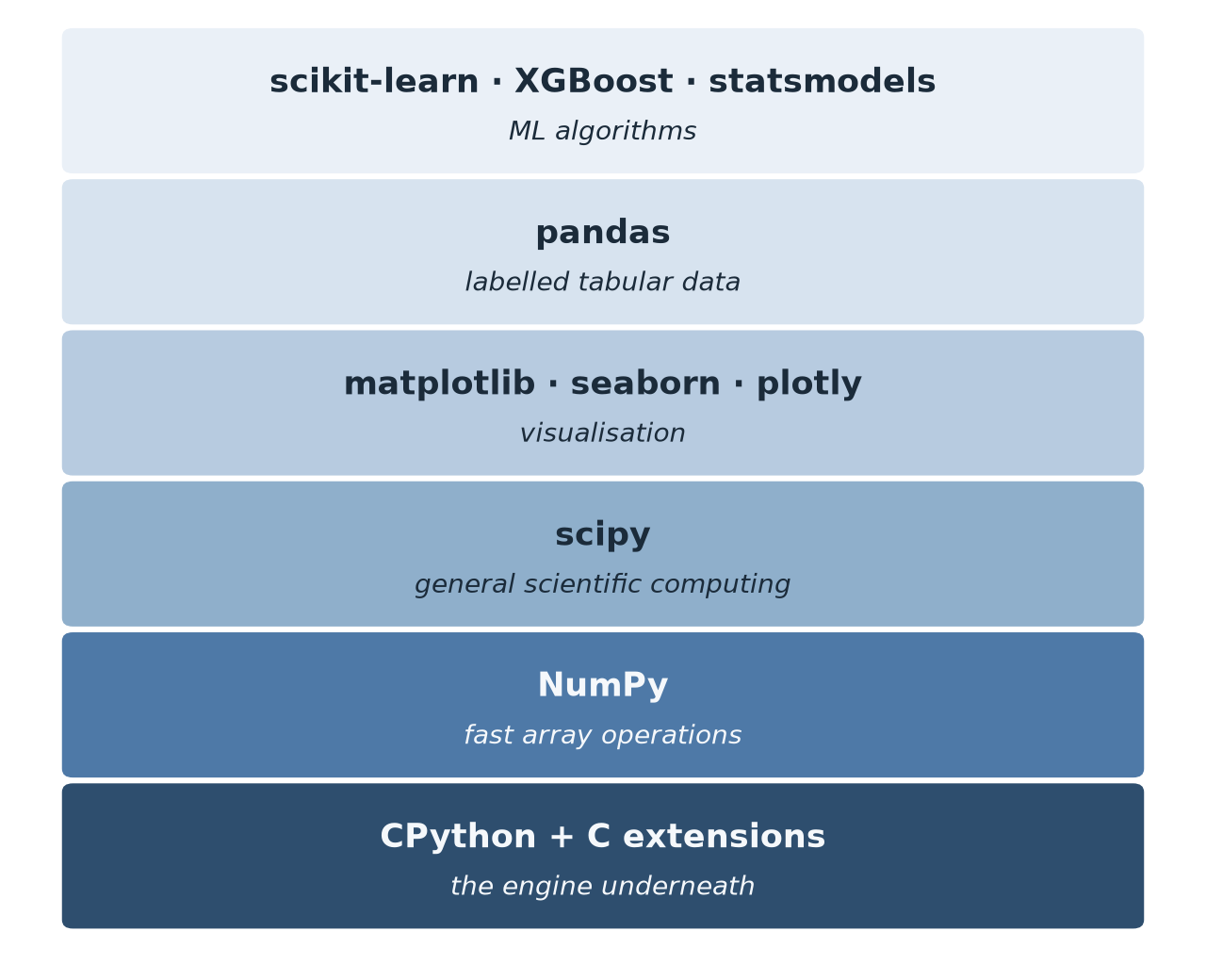
You don’t need to understand C to use NumPy. But you do need to understand NumPy to use pandas effectively. And you need pandas to use sklearn well. The abstractions are leaky in useful ways. pandas is built directly on NumPy arrays. Knowing that explains a great deal of pandas’ behaviour: why operations are fast, why .values and .to_numpy() exist, and why sklearn ultimately wants arrays, not DataFrames.
6.2.2 NumPy: Fast Arrays
Pure Python loops are slow for numerical work. Every iteration of for item in my_list: result += item * 2 forces the interpreter to check the type of item, look up the * operator, allocate a new integer object, and manage garbage collection. That overhead dominates once a list reaches a million elements. NumPy solves this by storing data in contiguous blocks of memory with a single fixed type: a float64 array is 64 bits per element, laid out in order. It implements operations on that memory in compiled C. That typically runs somewhere between 50 and 200 times faster than the equivalent Python loop, for simple elementwise operations like this.
The feature that makes this usable rather than just fast is broadcasting: NumPy applies operations between arrays of matching or compatible shapes without an explicit loop. array * 2, array_a + array_b, matrix @ vector all work element-wise or via broadcasting rules. All of them run in compiled code.
Broadcasting is NumPy’s rule for combining arrays of different shapes without writing a loop to line them up by hand. The simplest case: array + 5 adds 5 to every element. NumPy treats the single number 5 as if it were stretched into an array the same shape as array, without copying it in memory. The same idea extends to two arrays: adding a (3,) array to a (4, 3) array adds that one row to every one of the four rows. NumPy lines up their shapes from the right, and stretches any dimension that’s size 1, or missing, to match. Shapes that can’t be lined up this way raise a ValueError. Shapes that line up by accident broadcast without complaint, so a wrong-shaped array can still give a wrong answer silently.
Boolean indexing follows the same principle: array[array > threshold] filters without a loop, by first constructing a boolean mask (array > threshold) and then using it to select.
6.2.3 pandas: Labelled Tabular Data
NumPy arrays have no column names, no row labels, and no native concept of mixed types across columns. Every real dataset has all three. pandas supplies two structures on top of NumPy: a Series, a one-dimensional labelled array representing a single column, and a DataFrame, a two-dimensional labelled table whose columns can each hold a different type. The central concept is the index: every row carries a label, not just a position. That lets pandas align data from different sources automatically, support time-series-specific operations, and avoid the off-by-one errors that plague pure positional indexing. Because most DataFrame columns are NumPy arrays under the hood, pandas operations inherit NumPy’s speed. Any pandas Series can be dropped back down to a raw array with .to_numpy() whenever raw-array behaviour is needed.
6.2.4 matplotlib: The Low-Level Plotting Layer
matplotlib is the foundation of Python visualisation, and is deliberately imperative. It gives precise control over every element of a plot: axes, ticks, labels, colours, line styles, text. But it requires each of them to be spelled out, step by step. Every other visualisation library in the stack is built on top of it. When seaborn returns a plot, it is returning a matplotlib figure. When pandas’ .plot() is called, it is calling matplotlib internally. Fluency with matplotlib means any chart, regardless of which higher-level library generated it, can always be customised further.
6.2.5 seaborn: Statistical Visualisation
seaborn is a high-level wrapper around matplotlib, purpose-built for statistical data visualisation. It understands DataFrames natively, ships with better-looking defaults, and has built-in support for the chart types data scientists reach for constantly: distribution plots, regression plots, categorical comparisons, heatmaps, pairplots. In practice, matplotlib is for drawing, seaborn is for exploring data. For exploratory data analysis, seaborn is almost always the right starting point. For fine-grained custom charts, dropping to matplotlib is the right move.
6.2.6 scipy: Scientific Computing
scipy sits alongside NumPy and supplies algorithms that pure array operations can’t handle efficiently on their own: statistical tests, optimisation, signal processing, additional linear algebra, interpolation, integration. In day-to-day data science work, the module used most is scipy.stats (t-tests, chi-squared tests, and probability distributions), with scipy.optimize making occasional appearances (Chapter 4 covers optimisation in depth).
6.2.7 scikit-learn: The ML Algorithm Layer
scikit-learn is probably the most considered library in the ecosystem. Its defining feature is a consistent API that every estimator follows: .fit(X, y) learns from data. .predict(X) generates predictions for supervised models. .transform(X) transforms data for preprocessing steps. .fit_transform(X) does both in one call. .score(X, y) evaluates performance. Once LogisticRegression is understood, RandomForestClassifier is essentially already understood: same .fit(), same .predict(), same .score(). This consistency pays off more than it looks. The cost of learning a new algorithm in sklearn is mostly the cost of understanding the algorithm itself. sklearn also supplies preprocessing utilities (scaling, encoding), cross-validation, evaluation metrics, and pipelines that chain multiple steps into a single object.
6.2.8 Jupyter Notebooks: Literate Computing
A Jupyter notebook mixes live code, output (including charts), and markdown text in one document. The idea is older than Jupyter itself. Donald Knuth called this literate programming in 1984: write the code and the explanation of the code as a single interleaved document, meant to be read by a person first and a computer second. A notebook is that idea, running, decades later. It is the standard environment for data science because it makes exploration natural: run a cell, see the result, adjust, run again. A notebook doubles as a communication artefact. It can be shared with someone who doesn’t read Python, and they can still follow the narrative and understand the findings. The trade-off is that notebooks encourage non-linear execution: running cells out of order. That produces hidden state bugs that aren’t visible in the code as written. The discipline that prevents this: restart the kernel and run all cells top to bottom before treating any result as final.
6.3 Trade-offs and Limits
This stack excels at rapid prototyping and exploration, and at tabular data of any size that fits in memory. It’s good for sharing work with colleagues through notebooks. It also gives access to almost every classical ML algorithm ever published through one consistent interface. It struggles in three situations. Datasets larger than available RAM, where Dask, Spark, or a cloud-native tool is needed instead. Real-time production serving, where a dedicated serving framework replaces ad hoc notebook code (Book 2, Chapter 23 covers this in depth). Mobile or edge deployment, where LiteRT (formerly TensorFlow Lite) or ONNX are the right tools rather than the full stack. None of these are flaws in the libraries. They’re outside the problem this stack was built to solve: interactive, in-memory, exploratory analysis and modelling.
6.4 Procedures
Procedure 6.1 (Install and Verify the Stack). When to use: at the start of any new project or environment, before writing analysis code.
# Option A -- pip (minimal, exact control)
# pip install numpy pandas matplotlib seaborn scipy \
#     scikit-learn jupyter

# Option B -- conda (recommended for reproducibility)
# conda create -n dsenv python=3.11
# conda activate dsenv
# conda install numpy pandas matplotlib seaborn scipy \
#     scikit-learn jupyter

# Option C -- check an existing environment
import numpy, pandas, matplotlib, seaborn, scipy, sklearn
print(numpy.__version__, pandas.__version__, sklearn.__version__)
What to look for: a ModuleNotFoundError almost always means the wrong environment is active, not that the package is missing system-wide. Check which python / conda info --envs before reinstalling anything.
Procedure 6.2 (Convert Between NumPy Arrays and pandas DataFrames). When to use: scikit-learn’s estimators accept NumPy arrays; real data usually lives in a DataFrame first, so conversion happens at the fit/predict boundary.
import numpy as np
import pandas as pd

# DataFrame -> NumPy array
df = pd.DataFrame({'a': [1, 2, 3], 'b': [4, 5, 6]})
arr = df.to_numpy()            # (3, 2)

# NumPy array -> DataFrame
arr = np.array([[1, 2], [3, 4], [5, 6]])
df = pd.DataFrame(arr, columns=['col_a', 'col_b'])

# Series <-> 1D array
arr_1d = df['col_a'].to_numpy()
s = pd.Series(arr_1d, name='col_a')
Common mistake: scikit-learn raises a warning if a model is fit on a DataFrame with named features and later passed a plain array, or vice versa. Pick one representation per pipeline and stay consistent through the whole fit/predict cycle.
Procedure 6.3 (Plot Directly from a DataFrame). When to use: quick exploratory plots, before setting up matplotlib axes by hand is worth the effort.
import matplotlib.pyplot as plt

# line
df['value'].plot(title='My Value Over Time')
# bar
df.groupby('category')['value'].mean().plot(kind='bar', rot=0)
# histogram
df['age'].plot(kind='hist', bins=20, edgecolor='white')
# scatter
df.plot(kind='scatter', x='feature_a', y='feature_b', alpha=0.5)

plt.tight_layout()
plt.show()
Procedure 6.4 (Use scikit-learn’s Consistent fit/predict/score API). When to use: every time any sklearn estimator is fit. The five-method pattern never changes across algorithms.
from sklearn.neighbors import KNeighborsClassifier
from sklearn.preprocessing import StandardScaler
from sklearn.model_selection import train_test_split
from sklearn.metrics import accuracy_score

X_train, X_test, y_train, y_test = train_test_split(
    X, y, test_size=0.2, random_state=42
)

model = KNeighborsClassifier(n_neighbors=5)
model.fit(X_train, y_train)              # learn
y_pred = model.predict(X_test)           # predict
print(accuracy_score(y_test, y_pred))    # evaluate
Common mistake: fitting a scaler or encoder on X_test rather than only on X_train. The scaler must learn its mean and standard deviation exclusively from training data, then apply that same transform to test data:
scaler = StandardScaler()
# fit ON train, transform train
X_train_scaled = scaler.fit_transform(X_train)
# transform test with the SAME scaler
X_test_scaled = scaler.transform(X_test)
Fitting the scaler on X_test (or on the full dataset before splitting) leaks test-set statistics into training and silently inflates reported performance. The model looks better than it is, with no error raised to signal it.
Procedure 6.5 (Diagnose Common Stack Errors). When to use: when an error message doesn’t obviously point at its own cause.
| Error / symptom | Most likely cause | Fix |
|---|---|---|
ModuleNotFoundError: No module named 'numpy' |
Wrong environment active | Activate the right env, then reinstall |
ValueError: Input contains NaN |
sklearn received missing values | Clean data first (Chapter 7) |
DataConversionWarning: A column-vector y was passed |
y has shape (n, 1) not (n,) |
y.ravel() or y.squeeze() |
| Plot is blank / not showing | plt.show() called before the data-plotting calls |
Move plotting calls above plt.show() |
seaborn hue not working |
The hue column contains NaN values |
df.dropna(subset=['hue_col']) first |
6.5 Worked Example
The tutorial notebook behind this chapter is a tour through the whole stack, on two real, bundled datasets: seaborn’s Titanic passenger list and scikit-learn’s iris flower measurements. Three moments from it are worth walking through in detail, because each one makes a claim from the Exposition concrete with real numbers.
The first is the NumPy-versus-Python-loop speed claim. Doubling one million elements with a Python list comprehension versus NumPy’s vectorised multiplication, timed directly:
import numpy as np
import timeit

N = 1_000_000
py_list = list(range(N))
np_array = np.arange(N, dtype=np.float64)

t_py = timeit.timeit(
    '[x * 2 for x in py_list]', globals=globals(), number=5
) / 5
t_np = timeit.timeit(
    'np_array * 2', globals=globals(), number=5
) / 5
print(f'Python loop: {t_py*1000:.2f} ms')
print(f'NumPy:       {t_np*1000:.3f} ms')
print(f'Speedup:     {t_py/t_np:.0f}x')
On this machine, the Python loop takes roughly 27.7 ms and the NumPy operation roughly 0.24 ms, a 117x speedup, well within the “50-200x” range this chapter’s Exposition claims, and a difference that only grows as array size grows further.
The second moment combines pandas and scipy on the Titanic dataset (891 passengers, 15 columns). A grouped aggregation answers a real question (did survival rate depend on passenger class and sex?) in one line:
pivot = df.pivot_table(
    values='survived',
    index='pclass',
    columns='sex',
    aggfunc='mean',
)
print(pivot.round(2))
The result: first-class women survived at 97%, first-class men at 37%. By third class those numbers fall to 50% and 14% respectively. Class and sex both mattered, and mattered together. A single-dimension groupby would have hidden that. A natural follow-up question (did survivors pay more?) is answered with a two-sample t-test:
from scipy import stats

survivors = df[df['survived'] == 1]['fare'].dropna()
non_survivors = df[df['survived'] == 0]['fare'].dropna()

t_stat, p_value = stats.ttest_ind(survivors, non_survivors)
print(f'Survivor mean fare:     £{survivors.mean():.2f}')
print(f'Non-survivor mean fare: £{non_survivors.mean():.2f}')
print(f't = {t_stat:.2f}, p = {p_value:.2e}')
Survivors paid £48.40 on average against £22.12 for non-survivors, with t = 7.94 and p ~ 6.1e-15, from the default pooled-variance test. (Chapter 9’s Welch test, which doesn’t assume equal variances, gives p ~ 2.7e-11.) That’s far below the usual 0.05 threshold, so the fare gap is not plausibly due to chance. Fare correlates strongly with class, and class correlates strongly with survival. So this single number is surfacing the same class effect the pivot table showed directly. That’s a reminder that a significant p-value tells you a difference is unlikely to be chance, not what’s causing it.
The third moment is the scikit-learn API pattern, applied to the classic iris dataset (150 flowers, 4 features, 3 species):
from sklearn.datasets import load_iris
from sklearn.neighbors import KNeighborsClassifier
from sklearn.model_selection import train_test_split
from sklearn.metrics import accuracy_score

iris = load_iris(as_frame=True)
X_train, X_test, y_train, y_test = train_test_split(
    iris.data, iris.target, test_size=0.2, random_state=42
)

model = KNeighborsClassifier(n_neighbors=5)
model.fit(X_train, y_train)
y_pred = model.predict(X_test)
print(f'Accuracy: {accuracy_score(y_test, y_pred):.0%}')
With 120 training and 30 test samples, this particular split scores 100% accuracy. Iris is a famously easy, well-separated dataset. That’s exactly why it’s a good first dataset for learning the API pattern, rather than learning about model performance. Chapter 11 returns to k-Nearest Neighbours, on harder data, where accuracy stops being a foregone conclusion.
6.6 History and Further Reading
Thakur’s Ch. 1 sets up the working environment used throughout his book. It’s a good companion to this chapter’s Procedure 6.1 (Thakur 2020). Burkov’s Ch. 2 gives the same core concepts, vectors, matrices, functions, from the mathematical-notation side rather than the code side. It’s useful for connecting this chapter to Chapter 3’s formalism (Burkov 2019). Beyond the bibliography, the official NumPy quickstart at numpy.org and pandas’ “10 Minutes to pandas” guide are both worth reading directly. They’re as short as they claim to be, and more precise on edge cases (broadcasting rules, index alignment) than any secondary summary.
6.7 How This Connects
This chapter builds on ordinary Python fluency (lists, dicts, functions, pip), which this book treats as a prerequisite rather than a chapter of its own. It enables essentially everything that follows. Every remaining chapter in this book uses NumPy, pandas, and scikit-learn as its working vocabulary, the way Chapter 2 used pandas and sklearn.model_selection without pausing to introduce them. It is often confused with PyTorch and TensorFlow. Those are deep learning frameworks, covered starting in Book 2. They sit alongside this stack rather than inside it: a production system often uses pandas for data wrangling and scikit-learn for a baseline model, even when the final model is a neural network.
6.8 Exercises
[W] Using the layered-stack idea from this chapter’s Exposition, explain in one or two sentences why learning pandas well requires understanding NumPy, but not the other way around.
[W] State in one sentence each what
.fit(),.transform(), and.predict()do in the scikit-learn API pattern. Identify which of the three should never be called on test data.[A] Using Listing 6.6 as a template, measure the speedup of
np.sqrtover an equivalent Python loop (usingmath.sqrt) on an array of 500,000 elements, and report the ratio you observe.[A] Using Listing 6.7’s approach, compute survival rate by passenger class and
embark_towninstead of class and sex. Report which single (class, port) combination has the lowest survival rate.[A] Reproduce Listing 6.8, but compare passenger age between survivors and non-survivors instead of fare. Is the difference statistically significant at ? Which group is older on average?
[E] Procedure 6.4’s common mistake describes fitting a scaler on test data. Write two or three sentences explaining what would go wrong with a reported accuracy number if this mistake were made silently on a real project, and why no exception would be raised to catch it.
[E] A colleague proposes dropping pandas entirely and working with raw NumPy arrays “for speed” on a project with twenty columns of mixed numeric and categorical data. Using this chapter’s Trade-offs section, write the two or three sentence argument against this.
[R] Read the NumPy quickstart mentioned in this chapter’s Further Reading. Find one broadcasting rule this chapter’s Exposition did not discuss. Describe a data science situation where getting that rule wrong would silently produce an incorrect result rather than an error.
6.9 Mental Model
Think of the ecosystem as a toolbox with layers of abstraction. NumPy is the raw material. pandas is the workbench. matplotlib and seaborn are the drafting table. scikit-learn is the instrument kit. Going below NumPy is rarely necessary. pandas and scikit-learn will be used in essentially every project in this book. Knowing which layer a problem lives in is most of the battle in solving it quickly.