Chapter 9
Exploratory Data Analysis & Visualisation
Most modelling failures are not algorithmic. They are about what the data scientist failed to notice. A data scientist ships a model without noticing the target is heavily imbalanced, that two features are nearly redundant, or that a column silently changed units after a database migration. Exploratory Data Analysis (EDA) is the discipline that catches these problems before they become modelling problems. A structured, repeatable way of understanding a dataset before any modelling decision is made. It is not a step performed once. It is a mindset that a data scientist returns to after every surprising result. Every new feature. Every model iteration. This chapter builds that mindset into a repeatable sequence: look at each variable alone, look at pairs of variables, look at everything together, and write down what surprised you.
9.1 Motivation
EDA is a structured conversation with a dataset. The data scientist asks questions and lets the data answer, in a natural progression:
- What do I have? Shape, types, nulls, duplicates.
- What does each variable look like on its own? Distributions, outliers, skew.
- How do variables relate to each other? Correlations, conditional distributions.
- How do variables relate to the target? The most modelling-relevant question.
- What surprised me? The important question, asked last on purpose: only once the first four are answered is there enough context to recognise a genuine surprise.
There is no fixed script for EDA. The path is determined by what the data shows at each step. A surprising distribution at the univariate stage sends the analysis back to the data source. An unexpected correlation at the bivariate stage generates a hypothesis worth testing before any model is trained.
9.2 Exposition
9.2.1 Univariate Analysis
Univariate analysis examines one variable in isolation. For numeric variables, four properties matter. Central tendency: mean and median. If they diverge, the distribution is skewed. Spread: standard deviation and interquartile range. A spread near zero means the variable is nearly constant and gives a model little to use. Shape: bell-shaped, skewed, bimodal, or uniform. Outliers: extreme values that could be data-entry errors, or unusual, informative cases. For categorical variables, the properties that matter are different. Cardinality: how many unique values. A free-text column with thousands of unique values needs different treatment than a five-level category. Frequency distribution: is one category dominant enough to make the variable nearly constant? Rare categories: values so infrequent that no model can learn a reliable pattern from them.
9.2.2 Bivariate Analysis
Bivariate analysis examines two variables together. The right chart depends on the types involved.
- Two numeric variables. A scatter plot shows the relationship shape directly. A correlation coefficient summarises its strength: Pearson correlation for linear relationships, Spearman correlation for monotonic-but-non-linear ones.
- A numeric variable against a categorical one. Box plots or violin plots show whether the numeric distribution shifts across categories. If it does, the categorical variable carries information.
- Two categorical variables. Cross-tabulations and stacked bar charts reveal whether knowing one tells you something about the other.
The most important bivariate analysis in a modelling context is any variable against the target: does this feature’s distribution differ between target classes, or correlate with target values? If it doesn’t, the feature is a weak candidate for the model regardless of what it measures, or how important the customer thinks it is.
9.2.3 Multivariate Analysis
Multivariate analysis looks at three or more variables simultaneously. A pairplot (seaborn’s pairplot) draws a scatter plot for every pair of numeric variables at once, with each variable’s own distribution on the diagonal, coloured by a categorical variable of interest. It’s the fastest way to see a dataset’s full correlation structure in one figure. A correlation heatmap shows the Pearson correlation between every pair of numeric variables at a glance: values near ±1 flag strong linear relationships, values near 0 mean no linear relationship. Critically, a pair correlated above roughly 0.95 is close to redundant. Including both in a model rarely helps and sometimes hurts.
9.2.4 The EDA Mindset
The most valuable output of an EDA session is not a chart. It is a written list of hypotheses and surprises: things that didn’t match expectations. Leads worth following up. Modelling decisions the data is suggesting. Writing these down as they arise, instead of trusting memory, is what turns EDA into a narrative that connects to the feature engineering decisions of Chapter 14.
9.3 Trade-offs and Limits
How much EDA is enough? Enough to answer these questions:
- Are there data quality issues that need cleaning?
- Which features look promising?
- Are there obvious feature engineering opportunities?
- Is the target variable behaving as expected?
Going further than that risks data snooping: learning so much about a dataset, including its eventual test set, that later feature choices are implicitly optimised for data the model should never have seen. Running full EDA on a complete dataset before any train/test split is a common mistake for exactly this reason: patterns discovered that way may not hold on new data.
A second trade-off is visualisation versus summary statistics. Charts reveal shapes that statistics can hide entirely. The classic example is Anscombe’s quartet, four datasets with identical means, variances, and correlation coefficients but visibly different shapes when plotted. The rule is to visualise, even when the summary numbers look informative. A boxplot alone, for instance, can make a bimodal distribution look identical to a unimodal one. Boxplots show quartiles, not shape.
The same trick is easy to reproduce with fresh data. That makes the point more easily than quoting Anscombe’s original numbers: construct four datasets from scratch, one point at a time, so that all four end up with the same mean, spread, and correlation.
import numpy as np

rng = np.random.default_rng(11)
x = np.array([2, 4, 5, 7, 8, 9, 10, 11, 12, 13, 14, 16, 17, 18, 20], dtype=float)

# A: a genuine linear relationship, plus noise
y_linear = 0.60 * x + 2.6 + rng.normal(0, 2.9, len(x))
target_mean, target_std = y_linear.mean(), y_linear.std(ddof=1)

def match_stats(y_raw, mean, std):
    """Rescale y_raw to a target mean and std. An affine rescale like
    this changes nothing about the shape, or the correlation with x."""
    z = (y_raw - y_raw.mean()) / y_raw.std(ddof=1)
    return z * std + mean

# B: a curve, not a line
y_curved_raw = -0.0644 * (x - 13.97) ** 2 + 40 + rng.normal(0, 0.5, len(x))
y_curved = match_stats(y_curved_raw, target_mean, target_std)

# C: the same line as A, with one point pulled far off it
y_outlier_raw = 0.60 * x + 2.6 + rng.normal(0, 0.15, len(x))
y_outlier_raw[3] += 9.74
y_outlier = match_stats(y_outlier_raw, target_mean, target_std)

# D: x is nearly constant except for one high-leverage point
rng2 = np.random.default_rng(1186)
x_leverage = np.full(len(x), 9.681)
x_leverage[:-1] += rng2.normal(0, 0.05, len(x) - 1)
x_leverage[-1] = 9.681 + 20.79
x_leverage = match_stats(x_leverage, x.mean(), x.std(ddof=1))

y_leverage_raw = target_mean + rng2.normal(0, 0.4, len(x))
y_leverage_raw[-1] = 11.896
y_leverage = match_stats(y_leverage_raw, target_mean, target_std)
Running that against the actual generated data confirms the match: all four datasets land at mean , mean , , , and , agreeing to two decimal places. Figure 9.1 plots all four, each with the identical best-fit line drawn on top.
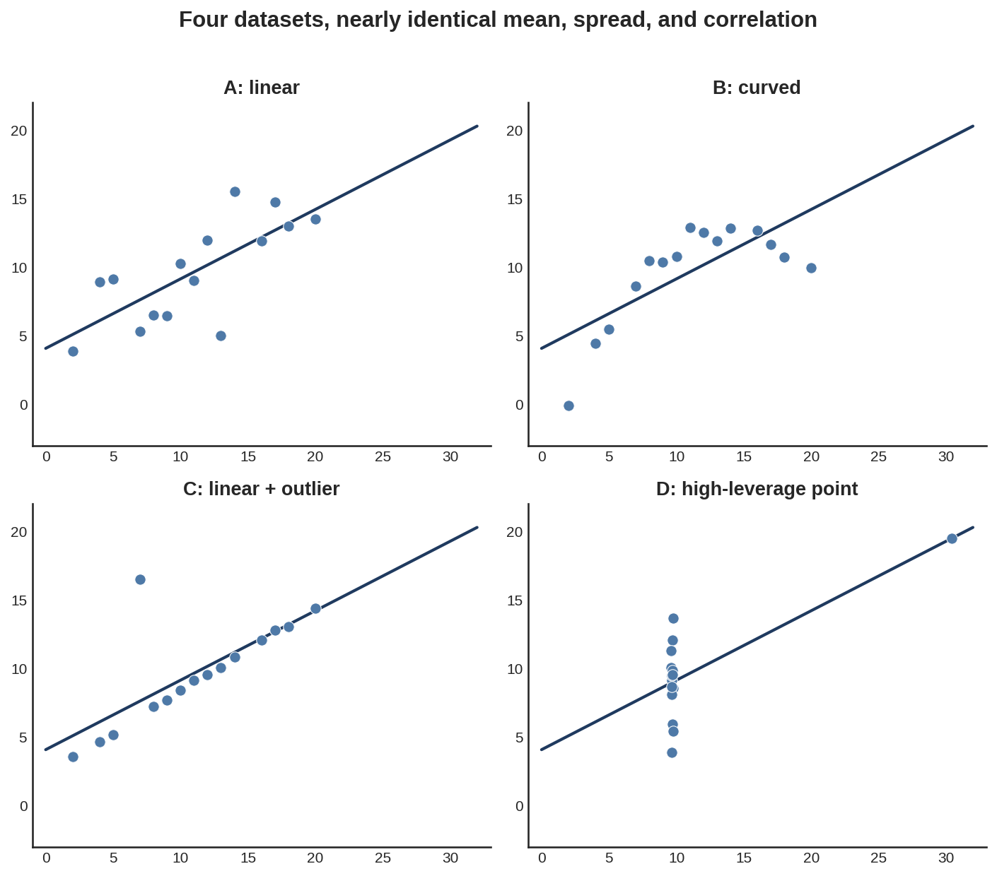
Panel A is the honest linear relationship the summary statistics describe. Panel B is a curve, not a line, that happens to produce the same correlation coefficient over this x-range. Panel C is the same line as A with a single point dragged far off it. Panel D is barely a relationship at all: fourteen points stacked at almost the same x-value, with one distant point single-handedly generating the entire correlation. A table of summary statistics reports the same four rows for all of them. Only the chart tells them apart.
9.4 Procedures
Procedure 9.1 (Profile a New DataFrame Fast). When to use: the first five minutes with any new dataset, before writing a single line of analysis.
import pandas as pd

def quick_profile(df: pd.DataFrame) -> None:
    print(f"Shape: {df.shape[0]} rows x {df.shape[1]} columns")
    print(f"\nDtypes:\n{df.dtypes.value_counts()}")
    print(f"\nDuplicate rows: {df.duplicated().sum()}")

    missing = df.isnull().sum()
    missing = missing[missing > 0].sort_values(ascending=False)
    if len(missing):
        pct_missing = (missing / len(df) * 100).round(1)
        print(f"\nColumns with missing values:\n{pct_missing}")
    else:
        print("\nNo missing values.")

    print(f"\nNumeric summary:\n{df.describe().T}")

quick_profile(df)
Common mistake: running .describe() and stopping there. Summary statistics hide shape. Always follow up with a histogram, per Anscombe’s quartet above.
Procedure 9.2 (Visualise the Missing-Value Pattern). When to use: immediately after .info() reveals nulls, to determine whether they are random or structural, e.g. a whole block of rows from one data source.
import matplotlib.pyplot as plt
import seaborn as sns

fig, ax = plt.subplots(figsize=(12, 4))
sns.heatmap(
    df.isnull(),
    yticklabels=False,
    cbar=False,
    cmap='viridis',
    ax=ax,
)
ax.set_title('Missing Value Map (bright = missing)')
plt.tight_layout()
plt.show()
Procedure 9.3 (Plot a Distribution). When to use: for every numeric column, before deciding on transforms or outlier handling.
fig, axes = plt.subplots(1, 2, figsize=(12, 4))

sns.histplot(
    df['fare'].dropna(), kde=True, ax=axes[0], color='#4E79A7'
)
axes[0].axvline(
    df['fare'].mean(), color='red', linestyle='--', label='mean'
)
axes[0].axvline(
    df['fare'].median(),
    color='orange',
    linestyle='--',
    label='median',
)
axes[0].legend()

sns.boxplot(x=df['fare'], ax=axes[1], color='#59A14F')
plt.tight_layout()
plt.show()
Common mistake: judging shape from a boxplot alone. Boxplots hide bimodality. A two-peaked distribution can look identical to a one-peaked one in a boxplot. Always pair it with a histogram or KDE.
Procedure 9.4 (Compute and Visualise a Correlation Matrix). When to use: once a dataset has more than a handful of numeric features and the full relationship structure needs to be seen at once.
import numpy as np

corr = df[numeric_cols].corr(method='pearson')

fig, ax = plt.subplots(figsize=(8, 7))
mask = np.triu(np.ones_like(corr, dtype=bool))
sns.heatmap(
    corr,
    mask=mask,
    annot=True,
    fmt='.2f',
    cmap='coolwarm',
    center=0,
    square=True,
    linewidths=0.5,
    ax=ax,
)
plt.tight_layout()
plt.show()

# Upper triangle only: each pair once, no self-pairs
upper = corr.abs().where(
    np.triu(np.ones_like(corr, dtype=bool), k=1)
)
pairs = upper.stack()
print(pairs[pairs > 0.95].sort_values(ascending=False))
Common mistake: using Pearson correlation on a monotonic-but-non-linear relationship (e.g. , where Pearson gives only about 0.69 for from 0 to 10) and reading the score as a weak relationship. Switch to method='spearman' when a non-linear monotonic relationship is suspected, or look at the scatter plot. A U-shape, such as over both negative and positive , scores near 0 on both. Only the scatter plot shows it.
Procedure 9.5 (Detect Outliers). When to use: after a distribution’s shape has already been seen visually, when a repeatable, code-based flag is needed instead of eyeballing.
from scipy import stats

def iqr_outliers(series: pd.Series, k: float = 1.5) -> pd.Series:
    """Flag values outside [Q1 - k*IQR, Q3 + k*IQR]."""
    q1, q3 = series.quantile([0.25, 0.75])
    iqr = q3 - q1
    lower, upper = q1 - k * iqr, q3 + k * iqr
    return (series < lower) | (series > upper)

def zscore_outliers(
    series: pd.Series, threshold: float = 3.0
) -> pd.Series:
    """Flag values more than `threshold` std devs from the mean."""
    z = np.abs(stats.zscore(series.dropna()))
    flags = pd.Series(z > threshold, index=series.dropna().index)
    return flags.reindex(series.index, fill_value=False)

mask = iqr_outliers(df['fare'])
print(f"{mask.sum()} outliers ({mask.mean():.1%} of rows)")
Common mistake: deleting every flagged outlier automatically. An outlier is a data point to investigate, not always to remove: it might be a data entry error worth fixing or deleting, or a rare but valid case worth keeping so the model can learn from it.
Procedure 9.6 (Compare a Numeric Variable Across a Categorical Target). When to use: the single most useful bivariate check before modelling: does this feature separate the target classes?
sns.kdeplot(
    data=df, x='fare', hue='survived', fill=True, common_norm=False
)

group_a = df[df['survived'] == 1]['fare'].dropna()
group_b = df[df['survived'] == 0]['fare'].dropna()
t_stat, p_value = stats.ttest_ind(
    group_a, group_b, equal_var=False
)
signal = (
    'likely informative' if p_value < 0.05 else 'weak/no signal'
)
print(f"p-value: {p_value:.2e}  ->  {signal}")
9.5 Worked Example
The tutorial notebook runs a complete, structured EDA on the Titanic passenger dataset (891 rows), following exactly the inspect-univariate-bivariate-multivariate-summarise structure above. The first inspection pass (Procedure 9.1 plus a missing-value heatmap, Listing 9.3) turns up three findings that shape everything downstream. age is missing for 19.9% of passengers, deck for 77.2%, and embarked/embark_town for 2 rows, few enough to drop safely. age needs imputation, and deck is close to unusable as a raw feature.
Target analysis comes next, because the target’s own behaviour constrains every metric choice later in the book. Only 38.4% of passengers survived. That’s a real but moderate imbalance, not the extreme kind that forces specialised techniques. But it’s still enough that accuracy alone would be a misleading metric (Chapter 2’s precision/recall framing).
Univariate analysis of the numeric features shows fare is heavily right-skewed (skewness : a small number of very expensive tickets stretch the distribution’s tail), while age is close to symmetric (skewness ). That skew is not a curiosity. It is the direct reason for log-transforming fare as a feature engineering step, an idea that resurfaces in Chapter 14.
Bivariate analysis against the target produces the chapter’s clearest signal:
df.groupby('sex')['survived'].mean()
df.groupby('pclass')['survived'].mean()
Run against the actual dataset, this returns a female survival rate of 74.2% against a male survival rate of 18.9%. That’s a 55-point gap. It makes sex the strongest single predictor in the dataset, visibly reflecting the historical “women and children first” evacuation policy. Passenger class shows the same kind of gradient: 63.0% survival in 1st class, 47.3% in 2nd, and 24.2% in 3rd. A Welch two-sample t-test comparing fares between survivors (mean £48.40) and non-survivors (mean £22.12) returns . That’s an overwhelmingly significant difference, consistent with fare acting as a proxy for class and cabin location.
The multivariate correlation pass (Procedure 9.4) against survived quantifies what the bivariate charts already suggested: pclass correlates at (higher class number, i.e. lower status, means lower survival), fare at , and age at only . That’s a weak marginal effect on its own, one that the notebook’s final multivariate step shows is misleading in isolation. Splitting age distributions by both class and survival status reveals a “children first” effect concentrated specifically in 1st and 2nd class, invisible in the marginal correlation and only visible once class is held fixed. That’s exactly the kind of pattern multivariate analysis exists to surface.
The notebook closes not with a chart but with a written five-point summary. Target imbalance requires imbalance-aware metrics. Sex is the strongest predictor. Class interacts with sex, rather than acting independently. Fare needs a log transform. And age’s 19.9% missingness should be handled with class-conditional median imputation, plus a was_missing indicator flag, rather than a single global fill value. That summary, not any individual chart, is the actual deliverable EDA hands to Chapter 14.
# SageMaker Data Wrangler generates a "Data Quality and
# Insights Report" (missing values, target leakage,
# duplicate rows, correlations, and outliers) without
# hand-written pandas.

# SageMaker Studio notebooks run the same pandas/matplotlib/
# seaborn workflow shown above, against data pulled directly
# from S3 or Athena:
import sagemaker
import pandas as pd

session = sagemaker.Session()
bucket = session.default_bucket()
# Requires s3fs installed
df = pd.read_csv(f"s3://{bucket}/raw/dataset.csv")
When to prefer SageMaker Data Wrangler (now part of SageMaker Canvas): when a shareable, automatically-generated data quality report is needed for stakeholders, or when the dataset is too large to comfortably profile locally. For a single analyst doing hands-on exploration, notebook pandas and seaborn are faster to iterate with.
9.6 History and Further Reading
Thakur’s early chapters give a practical, code-first approach to EDA that this chapter’s procedures closely mirror (Thakur 2020). Burkov’s second chapter covers the same territory from a more statistical angle, useful as a complementary framing of skewness, spread, and correlation (Burkov 2019, 15–25). Anscombe’s quartet, four datasets sharing identical means, variances, and correlations yet visibly different in shape, is worth a five-minute read on its own. It’s the single best reason for the “always visualise” rule in this chapter’s Trade-offs section. The seaborn documentation gallery is also worth bookmarking directly. Each example chart answers a different EDA question, and the plot type decision guide in Appendix A cross-references it.
9.7 How This Connects
This chapter builds on Chapter 7 (data must be clean before EDA is meaningful) and Chapter 6 (pandas, matplotlib, and seaborn are the toolkit EDA runs on). It enables Chapter 14 (feature engineering, where EDA’s findings become concrete transformations) and Chapter 11 (choosing which model families are worth trying, informed by what the data’s shape and relationships look like). It is often confused with feature engineering. But EDA is observing, while feature engineering is transforming. EDA’s job is to inform the engineering decisions Chapter 14 makes. Not to make them.
9.8 Exercises
[W] List the five questions this chapter’s EDA progression asks, in order, and explain in one sentence why “what surprises me?” is placed last rather than first.
[W] A dataset’s
agecolumn has a mean of 29.7 and a median of 28.0. What does the gap between them suggest about the distribution’s shape, and which single chart would confirm it?[A] Using Listing 9.2 as a starting point, run it against a dataset of your choosing and report which columns, if any, have more than 10% missing values.
[A] Using Listing 9.8’s grouping pattern, compute the Titanic survival rate broken down by
embarkedinstead ofsex. State whether the spread across categories looks large enough to be a useful feature.[A] Reproduce Listing 9.5’s “near-redundant pair” check on the Titanic numeric features (
survived,pclass,age,sibsp,parch,fare) and confirm whether any pair exceeds the 0.95 threshold.[E] The chapter found that
age’s marginal correlation withsurvivedwas only , yet a clear “children first” effect appeared once the data was split by class. Propose one other pair of Titanic features where you’d expect a similar effect, hidden in the overall numbers until the data is split. Explain your reasoning before checking it.[E] A colleague proposes running full EDA, including test-set rows, before splitting the data, arguing “we’re just looking, not modelling yet.” Using this chapter’s data-snooping discussion, write two or three sentences explaining what could go wrong.
[R] Read about Anscombe’s quartet (or its modern descendant, the “Datasaurus Dozen”). Pick one of the four Anscombe datasets. Describe, without plotting it, what summary statistics alone would have told you, and what they would have hidden.
9.9 Mental Model
EDA is journalism for datasets. The data scientist is investigating a story: gathering evidence, following leads, being surprised by what turns up, and then writing up findings in a way that helps someone else make a decision. That “someone else” is often future-you, deciding how to build the model.