Chapter 3
Maths Foundations: Statistics, Probability & Linear Algebra
Every machine learning algorithm is, underneath its API, a small set of mathematical ideas wearing a Python trenchcoat. Those ideas are a probability that expresses uncertainty, a statistic that summarises a sample, or a matrix operation that transforms a dataset. None of this requires re-deriving proofs from first principles. But it does require some fluency. You need to read an equation without flinching and notice when a model’s assumptions don’t match the data. You also need to explain to a customer why a result means what it means rather than what they hoped it meant. This chapter covers the three branches of mathematics that recur throughout the rest of this book: probability, statistics, and linear algebra. Not as abstract theory. As the specific vocabulary the following seventeen chapters assume. By the end, a single worked thread ties them together: the closed-form solution to linear regression. That’s simultaneously a statistics problem (minimise squared error), a linear algebra computation (solve a matrix equation), and the first model most of this book’s later classifiers and regressors generalise.
3.1 Motivation
Three older fields fuse into what we call data science. Probability is the calculus of uncertainty. Statistics is the practice of summarising data and drawing defensible inferences from it. Linear algebra is the language for representing and transforming structured data at scale. Most classifiers compute a probability underneath, even when the output is dressed as a class label. Most of exploratory data analysis is applied statistics, whether or not the word “statistics” ever appears in the code. And every dataset is, mechanically, a matrix. Every model operation, from a single linear regression to a hundred-layer neural network, is some sequence of matrix operations applied to that matrix. Skipping this chapter doesn’t make these ideas go away. It just means meeting them later, embedded in a library, without the vocabulary to reason about what they, and by extension you, are doing.
3.2 Exposition
3.2.1 Probability
A probability is a number between 0 and 1 that quantifies how likely an event is. means always happens. means it never does. means it happens 30% of the time, in the long run, across repeated trials. Conditional probability, written , is the probability of given that is already known to be true. This is the most important operation in machine learning. “Given these features, what is the probability of this outcome?” is a conditional probability question, whether the model computing it is a logistic regression or a hundred-billion-parameter transformer.
Bayes’ Theorem ties conditional probabilities together and is probably the most important equation in the field:
In ML terms, is the evidence you observe (features) and is the hypothesis you care about (a label). is the prior: what you believed before seeing any evidence, typically the base rate at which occurs in the population. is the likelihood: how probable the evidence is, assuming the hypothesis is true. , the posterior, is what you want: the updated probability of the hypothesis after accounting for the evidence.
A concrete, and deliberately uncomfortable, example makes the theorem’s practical bite obvious. Suppose a disease has 1% prevalence in a population (). A diagnostic test has 99% sensitivity () and 95% specificity (, so ). If someone tests positive, what’s the probability they have the disease? Expanding the denominator with the law of total probability, , gives
Only 16.7%, despite a test that looks 99% accurate on paper. The base rate, the disease’s rarity, dominates the result. The population of healthy people is so much larger than the population of diseased people that even a small false-positive rate among the healthy majority swamps the true positives from the rare minority. This is the mechanism behind the “high accuracy but useless” trap discussed for class-imbalanced classifiers in Chapter 2: every time a model is evaluated on data where the positive class is rare, that evaluation is implicitly a Bayes’-theorem calculation.
3.2.2 Common Probability Distributions
A distribution describes the shape of randomness expected in a variable: which values are likely, which are rare, and how spread out they are. Four distributions recur constantly in ML work:
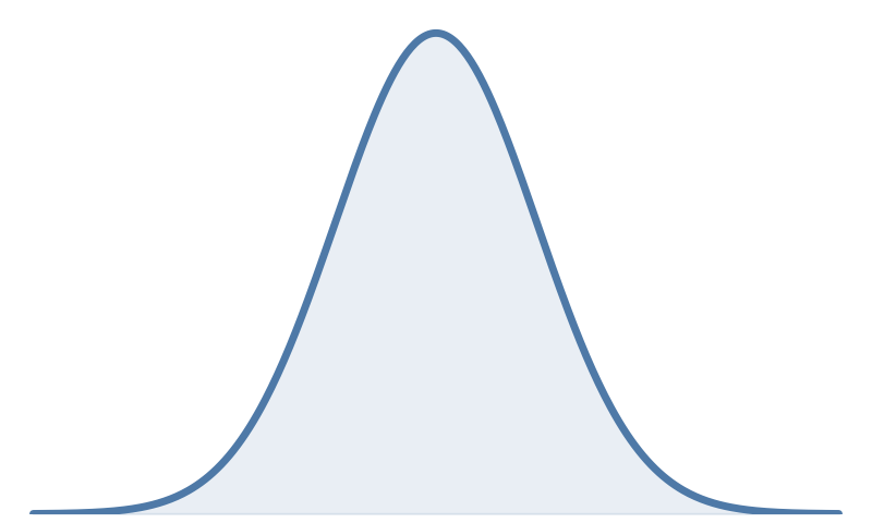
The Gaussian (Normal) distribution is the familiar bell curve, parameterised by mean and standard deviation , with density
It arises whenever many small, independent effects sum together. That’s the Central Limit Theorem’s signature. It’s why measurement error, model residuals, and many naturally occurring quantities are roughly Gaussian. Linear regression’s maximum-likelihood derivation assumes Gaussian residuals.
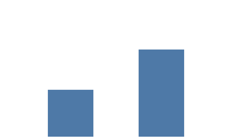
The Bernoulli distribution describes a single binary outcome: 1 with probability , 0 with probability . Every binary label in a classification problem (churned or not, fraud or not) is a Bernoulli random variable. Logistic regression is built explicitly around this assumption.
The Binomial distribution is the sum of independent Bernoulli trials (“how many successes in attempts?”), with mean and variance .
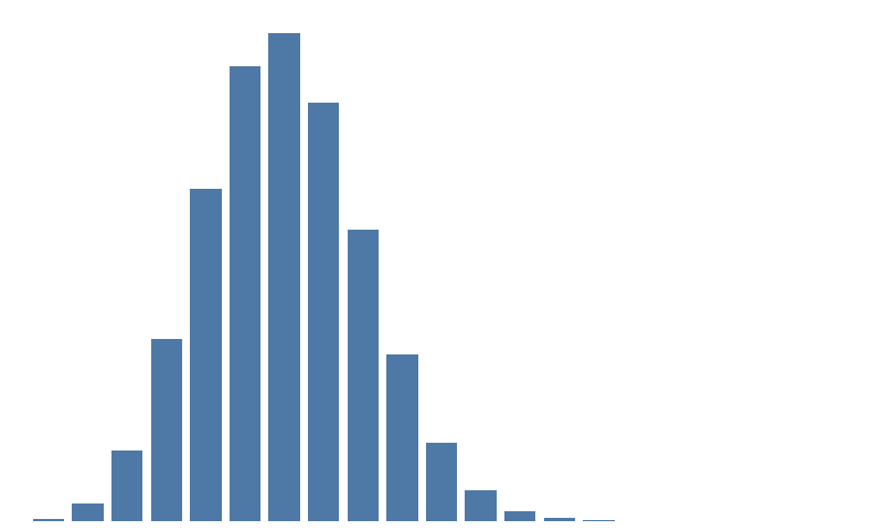
Compare that shape to the Gaussian a few paragraphs back. The resemblance isn’t accidental. A Binomial is a sum of independent Bernoulli trials. Summing many small independent effects is exactly the Central Limit Theorem’s territory. Once and are both comfortably above about 5, as they are in Figure 3.3, the Binomial looks Gaussian because it’s converging towards one. This is old news: Abraham de Moivre proved it in 1733, for the special case , long before anyone had named it the Central Limit Theorem. Pierre-Simon Laplace generalised the result to any in 1812. The result carries both their names today, the De Moivre-Laplace theorem: one of the oldest pieces of mathematics still doing daily work in this book.
The Poisson distribution describes counts of rare, independent events within a fixed interval (fraud events per day, machine failures per week), governed by a single rate parameter , with both mean and variance equal to .
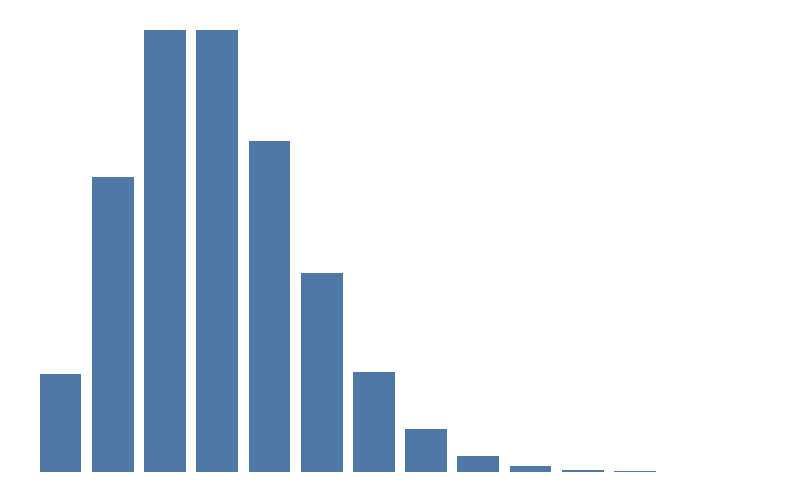
Choosing the wrong distributional assumption is a common modelling error. One example is fitting ordinary linear regression to count data with a long right tail, where a Poisson or negative-binomial model would fit far better. Another is assuming Gaussian residuals when the true error distribution is heavy-tailed. The distribution is a claim about the data-generating process. The model’s behaviour inherits that claim’s correctness or wrongness.
3.2.3 Statistics
Descriptive statistics summarise what a dataset looks like without invoking any inferential machinery. Most of this you already know from school, even if the vocabulary is new. The mean is the arithmetic average (what most people call “the average”) and is sensitive to outliers. The median is the middle value and is robust to them. When mean and median diverge by a lot, the underlying distribution is skewed.
You learned three averages in school: mean, median, and mode. Mean and median get most of the attention here. Mode, the most frequent value, rarely does, for good reason. On continuous data it’s often ill-defined: every exact value occurs with roughly zero probability, so an empirical mode depends entirely on how the data gets binned. Mean and median don’t have that problem. When it comes to optimisation: the mean is the single value that minimises the sum of squared deviations from it, and the median minimises the sum of absolute deviations. Mode isn’t the answer to any such minimisation problem. It’s just the most common value, and a distribution can have several of those, or none worth naming. Mode still earns its keep in specific spots: imputing missing categorical values, a “predict the most common class” baseline, and peak-finding in density estimation. It just isn’t part of this cluster of summary statistics, because it isn’t built the same way.
Variance, , measures average squared deviation from the mean. That divides by , the population version. pandas’ .std() and np.cov divide by instead, the sample version, which matters on small samples. Standard deviation, , restores the original units. Covariance measures how two variables move together: positive when they rise and fall in tandem, negative when one rises as the other falls. But its magnitude is scale-dependent, so it’s hard to interpret directly. Correlation (Pearson’s ) normalises covariance into the fixed range :
making it comparable across variables measured in entirely different units.
Hypothesis testing is the framework for deciding whether an observed pattern reflects something real or could plausibly be random chance. The procedure: assume no effect exists (the null hypothesis ). Compute how surprising the observed data would be under that assumption. Reject if the data is unlikely enough. The p-value is the probability, under , of observing data at least as extreme as what was observed. is the conventional cutoff for “statistically significant.” That’s a threshold chosen by convention, not derived from any deep principle. And it’s the most misused number in science.
Push on that threshold and it stops meaning much. Try enough subgroups, metrics, or stopping points on the same dataset, and something will clear by chance alone. That practice has a name: p-hacking, often unconscious rather than deliberate. That practice is a central cause of what’s now called the replication crisis. In 2015, the Open Science Collaboration tried to redo 100 published psychology studies and found only 36% produced a statistically significant result the second time. The original studies weren’t necessarily fraudulent. Most were the predictable output of researchers making reasonable-looking choices, one p-value at a time, until something crossed the line.
The trap: a small p-value means the data would be surprising if there were no effect, assuming you haven’t gone rooting around in the undergrowth for it. But it says nothing about whether that effect is large or practically meaningful. With enough data, a model improvement from 0.9000 to 0.9001 accuracy can register while being irrelevant to any business decision. A p-value should never be reported alone. It needs an accompanying effect size (such as Cohen’s , the standardised difference between two group means) and, ideally, a confidence interval, so that statistical significance and practical significance can be evaluated separately.
3.2.4 Linear Algebra
Two symbols show up constantly from here on. is the set of all real numbers: any number on the number line, positive or negative, with or without decimals. means “ordered lists of 7 real numbers,” so a customer vector living in just means it has 7 numeric features. means “is an element of,” or more plainly, “belongs to” or “is a member of.” reads as “ belongs to the set of all real-valued matrices with rows and columns.” That’s a formal way of saying “ is an matrix of real numbers.” Neither symbol does anything exotic. They’re set-theory notation borrowed to say precisely what shape and type of number is being talked about.
A vector is an ordered list of numbers. In ML, one row of a dataset (one data point) is a vector. A customer described by seven features (tenure, spend, ticket count, and so on) is a single point in . In code, a vector is a numpy array: fixed-length, one numeric type, built to support the arithmetic below directly.
A Python list looks like a vector but doesn’t behave like one. [1, 2, 3] + [4, 5, 6] concatenates into [1, 2, 3, 4, 5, 6], not [5, 7, 9]. A numpy array does the elementwise thing a vector needs: np.array([1, 2, 3]) + np.array([4, 5, 6]) gives [5, 7, 9]. Reaching for a list where an array belongs is one of the most common sources of silent, wrong-shaped bugs in early numpy code.
A matrix is a two-dimensional array of numbers. An entire dataset is a matrix: rows (observations) by columns (features), written .
The dot product of two vectors, , is the sum of their element-wise products. It is the fundamental operation behind prediction: a linear model’s output is the dot product between a feature vector and a weight vector. Concretely: if and , then . Multiply each pair of matching elements, then add the results. A tiny prediction looks the same. A customer with 5 months’ tenure and $80 monthly spend is the feature vector . A model’s learned weights might be . The prediction is . Every linear model prediction, no matter how many features, is this same operation done at larger scale.
Matrix multiplication generalises the dot product across many vectors at once (if is and is , then is ). Concretely: let and . Each entry of is a dot product: row of against column of . The top-left entry is row 1 of , , dotted with column 1 of , : . Working through all four entries the same way gives
Nothing new happened here. It’s the same multiply-then-add from the dot product example above, done four times, once per output entry. This single operation, chained repeatedly with non-linearities in between, is how every neural network layer transforms its input.
The transpose of a matrix, , flips rows and columns. It appears throughout ML’s closed-form solutions.
The identity matrix is the matrix equivalent of the number 1: square, with 1s down the main diagonal and 0s everywhere else, for example in two dimensions. Multiplying anything by it leaves that thing unchanged, , the same way multiplying a number by 1 leaves it unchanged.
The inverse of a square matrix satisfies : the matrix version of “a number times its reciprocal equals 1.” It exists only for square, non-singular matrices. In practice, computing directly is both slower and numerically less stable than solving a linear system with np.linalg.solve. Prefer np.linalg.solve whenever the goal is to solve , rather than to obtain as an object.
This explains several things that would otherwise be opaque rules of thumb. Feature scaling matters because dot products and distance metrics are sensitive to the raw magnitude of each feature. A feature measured in the tens of thousands (income) will dominate a distance calculation against a feature measured in single digits (age) unless both are normalised onto comparable scales. Principal Component Analysis, covered in a later chapter, works by finding the directions of maximum variance in the data matrix. That computation is, at its core, an eigendecomposition of the data’s covariance matrix.
And neural networks can approximate complex, highly non-linear functions precisely because they interleave linear (matrix multiplication) and non-linear (activation function) steps. The linear algebra provides the structure, the non-linearities provide the expressive power.
Multiplying a vector by a matrix usually changes both its direction and its length. An eigenvector of a matrix is a special vector that keeps its direction. The matrix only stretches or shrinks it, by a factor called the eigenvalue: . A simple case makes this concrete. Let . Applying to gives , which is just scaled by 2. Applying to gives , scaled by 3. Those two directions, and their scaling factors 2 and 3, are ’s eigenvectors and eigenvalues. An eigendecomposition finds all of a matrix’s eigenvectors and eigenvalues at once, breaking the matrix down into its fundamental stretch directions. This is exactly what PCA uses. The eigenvector with the largest eigenvalue points in the direction the data is most spread out in. That’s the definition of a principal component.
3.2.5 Linear Regression as a Matrix Equation
The simplest supervised model, linear regression, is where probability, statistics, and linear algebra meet. In matrix form, predictions are
where is the feature matrix, is the weight vector, and is the resulting vector of predictions. “Learning” here means finding the that minimises the sum of squared errors between and the true (a statistics objective). That minimisation has an exact, closed-form solution called the normal equations:
This is not an approximation. It’s not an iterative procedure. It is the exact minimiser, derivable in a few lines of calculus (Chapter 4 covers the calculus side properly). It is the same answer sklearn.linear_model.LinearRegression returns. sklearn gets there with a more numerically stable least-squares solver rather than forming , but the minimiser is the same. The Worked Example below verifies this by hand against the iris dataset and confirms the numpy and sklearn results agree to six decimal places.
3.3 Trade-offs and Limits
The depth of maths needed scales with the job at hand. Anywhere model uncertainty, calibration, or Bayesian methods are directly in play, the probability theory in this chapter is required. Murphy’s introductory text goes considerably further into formal probability than this chapter attempts. But for the large majority of day-to-day ML work, sklearn, XGBoost, and similar libraries do the underlying matrix algebra and optimisation internally. The practitioner’s job is not to re-derive the normal equations from scratch every time. The job is to have enough intuition that nothing the library does is surprising, and enough fluency to debug when results look wrong. A model that suddenly produces NaN predictions after a feature-scaling change, for instance, is far easier to diagnose with an intuition for numerical instability in matrix inversion than without one.
The p-value trap deserves its own note here because it recurs throughout applied statistics. Statistical significance is not the same claim as practical importance. Treating as a stopping condition (rather than one input alongside effect size and business context) is one of the most common statistical mistakes in industry data science, not just academic research.
3.4 Procedures
Procedure 3.1 (Compute and Interpret Correlation). When to use: during exploratory data analysis, to identify which features relate to the target and to each other.
import pandas as pd
import seaborn as sns
import matplotlib.pyplot as plt

r = df['feature_a'].corr(df['target'])
print(f"r = {r:.3f}")

corr = df.corr(numeric_only=True)

sns.heatmap(corr, annot=True, fmt='.2f', cmap='RdBu_r',
            center=0, vmin=-1, vmax=1, square=True)
plt.tight_layout()
plt.show()

corr_with_target = (
    corr['target']
    .abs()
    .sort_values(ascending=False)
)
print(corr_with_target.head(10))
Common mistake: correlation measures linear relationships only. A feature can carry strong non-linear predictive power while its Pearson sits near zero. Always inspect the scatter plot, not just the coefficient.
Procedure 3.2 (Test for Normality). When to use: before applying any statistical test that assumes Gaussian data: the t-test, ANOVA, or linear regression residual diagnostics.
from scipy import stats
import matplotlib.pyplot as plt

data = df['column_name'].dropna()

fig, axes = plt.subplots(1, 2, figsize=(10, 4))
axes[0].hist(data, bins=30)
axes[0].set_title('Histogram')
stats.probplot(data, plot=axes[1])
axes[1].set_title('Q-Q Plot (straight line = Gaussian)')
plt.tight_layout()
plt.show()

stat, p = stats.shapiro(data)          # best for n < 5000
print(f"Shapiro-Wilk: W={stat:.4f}, p={p:.4f}")
print("Gaussian" if p > 0.05 else "Not Gaussian")

stat, p = stats.normaltest(data)       # better for larger samples
print(f"D'Agostino-Pearson: p={p:.4f}")
If the data isn’t Gaussian, prefer median/IQR over mean/std for summaries. Use the Mann-Whitney U test instead of a t-test. Consider log-transforming a right-skewed variable with np.log1p.
Procedure 3.3 (Perform Core Matrix Operations in numpy). When to use: any time feature matrices need to be manipulated directly, or an ML operation needs to be implemented from first principles.
import numpy as np

A = np.array([[1, 2], [3, 4], [5, 6]])  # shape (3, 2)
B = np.array([[7, 8], [9, 10]])          # shape (2, 2)

A.T                # transpose, shape (2, 3)

# matrix multiply — ALWAYS use @, not np.dot, for 2D arrays
C = A @ B

v1 = np.array([1, 2, 3])
v2 = np.array([4, 5, 6])
v1 @ v2            # dot product = 1*4 + 2*5 + 3*6 = 32

M = np.array([[2.0, 1.0], [1.0, 3.0]])

# equivalent to M^{-1}, computed more stably
np.linalg.solve(M, np.eye(2))

# solves M @ x = b directly — prefer this over inv()
b = np.array([1.0, 2.0])
np.linalg.solve(M, b)

eigenvalues, eigenvectors = np.linalg.eig(M)   # used in PCA

np.linalg.norm(v1)               # L2 norm (Euclidean length)
np.linalg.norm(v1, ord=1)        # L1 norm (Manhattan distance)

X = np.random.randn(100, 5)      # (N, M) data matrix
w = np.random.randn(5)           # (M,) weight vector
y_hat = X @ w                    # (N,) predictions
Common mistake: M * M is element-wise multiplication, not matrix multiplication (M @ M). Mixing up * and @ on two matrices of the same shape produces a result that runs without error but is mathematically wrong.
Procedure 3.4 (Interpret a p-value Correctly). When to use: whenever reporting a statistical test result or evaluating a claim about model performance.
from scipy import stats
import numpy as np

group_a = df[df['group'] == 'A']['metric']
group_b = df[df['group'] == 'B']['metric']
t_stat, p_value = stats.ttest_ind(group_a, group_b)
print(f"t = {t_stat:.3f}, p = {p_value:.4f}")

# simple pooled std: fine when the groups are the same size
pooled_std = np.sqrt((group_a.std()**2 + group_b.std()**2) / 2)
cohens_d = (group_a.mean() - group_b.mean()) / pooled_std
# 0.2=small, 0.5=medium, 0.8=large
print(f"Cohen's d = {cohens_d:.3f}")
Common mistake: treating as proof of “no effect.” It only means “insufficient evidence of an effect,” which is a materially weaker claim. A related mistake is running many hypothesis tests and reporting only the ones that happen to clear (p-hacking). When testing hypotheses at once, apply a Bonferroni correction and use threshold instead.
Procedure 3.5 (Compute Summary Statistics by Group). When to use: understanding how a feature differs across classes, a standard step in exploratory data analysis.
(
    df.groupby('species')[numeric_cols]
    .agg(['mean', 'std', 'median'])
    .round(3)
)

# check for heteroscedasticity
df.groupby('species')['feature'].var()

df[numeric_cols].cov()

z_scores = (df[col] - df[col].mean()) / df[col].std()
outliers = df[z_scores.abs() > 3]
print(f"{len(outliers)} outliers in {col}")
3.5 Worked Example
The companion notebook builds a complete mathematical toolkit in three parts, each verifying a claim from the Exposition against real computation rather than leaving it as assertion.
Part 1 — the Law of Large Numbers and Bayes’ Theorem. Simulating 10,000 fair coin flips (np.random.binomial(1, p=0.5, size=10_000), seed 42) and tracking the running frequency of heads shows convergence towards the true probability, exactly as claimed. The observed frequency after all 10,000 flips is 0.4924, visibly closer to 0.5 than the frequency after only a handful of flips. The gap shrinks roughly as .
P_disease = 0.01
P_pos_given_dis = 0.99
P_neg_given_healthy = 0.95
P_pos_given_healthy = 1 - P_neg_given_healthy
P_healthy = 1 - P_disease

P_positive = (
    (P_pos_given_dis * P_disease)
    + (P_pos_given_healthy * P_healthy)
)
P_disease_given_pos = (P_pos_given_dis * P_disease) / P_positive

print(f"P(positive):                {P_positive:.3f}")
print(f"P(disease | test positive): {P_disease_given_pos:.1%}")
Running this gives P(positive) = 0.059 and P(disease | test positive) = 16.7%. That matches the Exposition’s hand-worked figure exactly. It’s confirmed independently by a direct simulation over 100,000 synthetic people, counting true and false positives directly rather than trusting the algebra alone.
Part 2 — full statistical analysis of the iris dataset. The classic four-feature, three-species iris dataset (150 rows) makes mean-vs-median skew concrete. petal length (cm) has mean 3.758 cm against median 4.350 cm, a difference of 0.592 cm. That’s by far the largest gap of the four features (the next largest, petal width, differs by only 0.101 cm). The reason: the dataset mixes three species whose petal lengths cluster in different ranges, producing a bimodal, not symmetric, overall distribution. The correlation matrix confirms the strongest linear relationship in the dataset is between petal length and petal width, at . That’s visibly higher than sepal length vs. petal length () or sepal length vs. petal width (). Running Shapiro-Wilk normality tests (Procedure 3.2) on each feature across all species combined rejects Gaussianity for sepal length (), petal length () and petal width (). That’s unsurprising, since mixing three species’ distributions produces multimodality. Restricting to setosa alone brings both sepal length () and sepal width () comfortably back into “consistent with Gaussian” territory. This illustrates that Shapiro-Wilk tests the sample actually given to it, not some platonic notion of the feature.
Part 3 — linear regression from scratch, verified against sklearn. Using petal length to predict petal width (Listing 3.7), solving the normal equations directly with np.linalg.solve produces:
X_raw = df[['petal length (cm)']].values
y = df['petal width (cm)'].values
# add bias column
X = np.column_stack([np.ones(len(X_raw)), X_raw])

XtX = X.T @ X
Xty = X.T @ y
w = np.linalg.solve(XtX, Xty)
print(f"Intercept (w0): {w[0]:.4f}")
print(f"Slope     (w1): {w[1]:.4f}")
w = [-0.3631, 0.4158], i.e. petal_width ~ -0.3631 + 0.4158 × petal_length. Fitting sklearn.linear_model.LinearRegression on the same data gives intercept -0.363076 and coefficient 0.415755. That matches the numpy result to six decimal places, confirming these are the same computation under two different names. The fitted model achieves and cm. Petal length alone explains close to 93% of the variance in petal width across all three species, with an average prediction error of about two millimetres. That’s a strikingly tight fit for a single-feature linear model. It’s a direct consequence of the correlation already observed in Part 2: for simple linear regression, is exactly ().
3.6 AWS SageMaker Notes
# SageMaker Data Wrangler provides a UI for
# statistical analysis at scale. For programmatic
# stats on datasets too large for local memory, use
# SageMaker Processing Jobs instead:

import sagemaker
from sagemaker.processing import ScriptProcessor

# processor = ScriptProcessor(
#     image_uri=...,
#     role=role,
#     instance_type='ml.m5.xlarge',
#     instance_count=1,
# )
# processor.run(code='stats_script.py', ...)
When to prefer SageMaker Processing: once a dataset no longer fits comfortably in local memory (roughly beyond 10 GB). Below that threshold, pandas and scipy running locally are faster to iterate with and cost nothing per run. Reach for managed infrastructure only once local computation is the bottleneck.
3.7 History and Further Reading
Murphy’s introductory volume gives the formal treatment this chapter deliberately keeps informal. Chapter 2 covers probability theory properly (joint, marginal, and conditional distributions). Chapter 3 covers estimation, hypothesis testing, and confidence intervals in full (Murphy 2022). The same book’s Appendix B is, in the author’s own words, exactly the depth of linear algebra review an ML practitioner needs, no more, no less (Murphy 2022). Burkov’s opening chapter is worth a quick pass for its notation conventions and its concise statement of the supervised learning setup. This chapter’s linear regression example builds on that setup directly (Burkov 2019, 1–10). This chapter keeps the linear algebra informal. For the fully rigorous treatment, Humpherys, Jarvis, and Evans’ Foundations of Applied Mathematics, Volume 1: Mathematical Analysis builds vector spaces axiomatically over arbitrary fields, rather than this chapter’s concrete starting point. It’s worth a look for exactly that contrast (Humpherys et al. 2017). Chu-Carroll’s Good Math is a different kind of companion. It’s not a probability or linear algebra text, but an accessible, narrative tour of number systems, logic, and computability. It gives the curious reader a broader sense of the mathematical foundations sitting underneath this chapter’s notation (Chu-Carroll 2013). Beyond formal texts, 3Blue1Brown’s “Essence of Linear Algebra” video series is widely regarded as the best available visual intuition for matrix operations. It gives geometric intuition for transposes, matrix multiplication as a transformation, and eigenvectors, in a way no amount of algebraic manipulation alone conveys.
3.8 How This Connects
This chapter builds on Chapter 2. With a defined ML problem in hand, this chapter supplies the mathematical language needed to describe precisely what that problem is optimising. It enables Chapter 4 (Calculus & Optimisation), which picks up exactly where the normal equations’ limitations leave off: most real models have no closed-form solution and need gradient descent instead. It also enables the supervised learning chapters later in this book, and the neural network chapters in Book 2. It’s often confused with a demand for mathematical expertise. What it requires is mathematical literacy: the ability to read an equation, recognise which operation it describes, and reason about what changing an input does to the output, not the ability to derive every result from a blank page.
3.9 Exercises
[W] Using the disease-test numbers from Listing 3.6, explain in your own words why comes out so much lower than the test’s 99% sensitivity would naively suggest.
[W] For each of the following, name the distribution (Gaussian, Bernoulli, Binomial, or Poisson) that best describes it, and justify your choice in one sentence: (a) whether a single email is spam; (b) the number of fraudulent transactions in a given hour; (c) the number of heads in 50 coin flips; (d) the measurement error of a sensor reading a stable physical quantity.
[A] Using Procedure 3.1 and the iris dataset, compute the correlation between
sepal width (cm)and every other feature. Which pair has the weakest (closest to zero) correlation, and does that match the intuition that sepal width is the “odd one out” of the four iris measurements?[A] Extend Listing 3.7 to use two features,
petal length (cm)andsepal length (cm), to predictpetal width (cm). You only need to change howX_rawis constructed. The normal-equations solve is unchanged. Report the new and state whether adding the second feature meaningfully improved the fit over the single-feature model.[A] Using Listing 3.4, run a two-sample t-test comparing
petal length (cm)betweensetosaandversicolorin the iris dataset. Report the p-value and Cohen’s , and state in one sentence whether the difference is both statistically significant and practically large.[E] A colleague reports “we found a statistically significant improvement, ” as the sole justification for shipping a model change. Using this chapter’s discussion of p-values and effect sizes, write the two or three follow-up questions you’d ask before agreeing the change should ship.
[E] Section “Linear Algebra” argues that feature scaling matters because dot products and distance metrics are sensitive to raw magnitude. Construct a small numeric example (two features, three or four data points) where an unscaled Euclidean distance calculation is dominated by one feature, and show the same calculation after standardising both features to mean 0 and standard deviation 1.
[R] Read Murphy’s Appendix B on linear algebra (Murphy 2022). Find one operation or concept covered there that this chapter didn’t mention, and explain in a short paragraph where it would become relevant later in this book (for instance, in the PCA or neural network chapters).
3.10 Mental Model
A dataset is a matrix. A model is a function that transforms that matrix into predictions. A training objective is an equation that measures how wrong those predictions are. Probability is the language that objective is usually expressed in. Statistics is how confidence in a result, or lack of it, gets quantified once the model exists. None of this requires being a mathematician. It requires being able to read these equations without flinching. From here on, every chapter in this book assumes exactly that.