Chapter 18
Regularisation
A model reaches 98% accuracy on training data and 72% on unseen test data. That’s a textbook overfit. The model learned the training set’s noise instead of its underlying signal. Regularisation is the primary tool for fighting this. It works by penalising model complexity during training. That pushes the model towards simpler explanations that generalise better, rather than more complex ones that memorise.
18.1 Motivation
A model with enough degrees of freedom can perfectly memorise any training set. More data helps, but it often isn’t available. You need to constrain how much the model is allowed to memorise. Regularisation adds a cost for complexity to the training objective. Instead of minimising prediction error alone, the model minimises prediction error plus a penalty for large or complex weights. Penalty terms for linear models, dropout for neural networks, depth limits for decision trees, early stopping for iterative training: all forms of regularisation. The form changes by model type. The underlying principle is the same across all of them.
18.2 Exposition
18.2.1 The Bias-Variance Trade-off
Chapter 11’s Bias-Variance Trade-Off section introduced this decomposition in full: . Regularisation trades a small increase in bias for a larger reduction in variance. The result is lower total error on unseen data.
18.2.2 Diagnosing with Learning Curves
The bias-variance trade-off is conceptual. A learning curve is how to see which side of it a model is on, before choosing whether to regularise, simplify, or collect more data. Train the model on increasing subsets of the training set (10%, 20%, and so on). At each size, record both training error and validation error, then plot both against training-set size. This is a different diagnostic from Chapter 4’s loss curve, which plots error against training epoch to check whether a model is converging. A learning curve asks a different question: would more data help?
If both curves converge to a similarly high error as training-set size grows, that’s high bias. The model is too simple for the signal in the data. No amount of extra data will help. A more flexible model or better features is the fix. If training error stays low while validation error stays higher, with a gap that persists (though usually narrows) as training-set size grows, that’s high variance. The model has the capacity to overfit. More data, or more regularisation, is the fix.
import numpy as np
from sklearn.model_selection import learning_curve
from sklearn.linear_model import LinearRegression
from sklearn.tree import DecisionTreeRegressor

rng = np.random.RandomState(42)
X = rng.uniform(0, 10, 400).reshape(-1, 1)
y = 3 * np.sin(1.5 * X.ravel()) + rng.normal(0, 0.5, 400)

train_sizes = np.linspace(0.1, 1.0, 10)
fig, axes = plt.subplots(1, 2, figsize=(12, 4.5))

for ax, model, title in [
    (axes[0], LinearRegression(), 'High bias: LinearRegression on a sine curve'),
    (axes[1], DecisionTreeRegressor(),
     'High variance: unconstrained DecisionTreeRegressor'),
]:
    ts, train_scores, val_scores = learning_curve(
        model, X, y, train_sizes=train_sizes,
        cv=5, scoring='neg_root_mean_squared_error',
    )
    ax.plot(ts, -train_scores.mean(axis=1), color='#4E79A7', marker='o',
            label='Training error')
    ax.plot(ts, -val_scores.mean(axis=1), color='#E15759', marker='s',
            linestyle='--', label='Validation error')
    ax.set_xlabel('Training set size')
    ax.set_ylabel('RMSE')
    ax.set_title(title)
    ax.legend()

plt.tight_layout()
plt.show()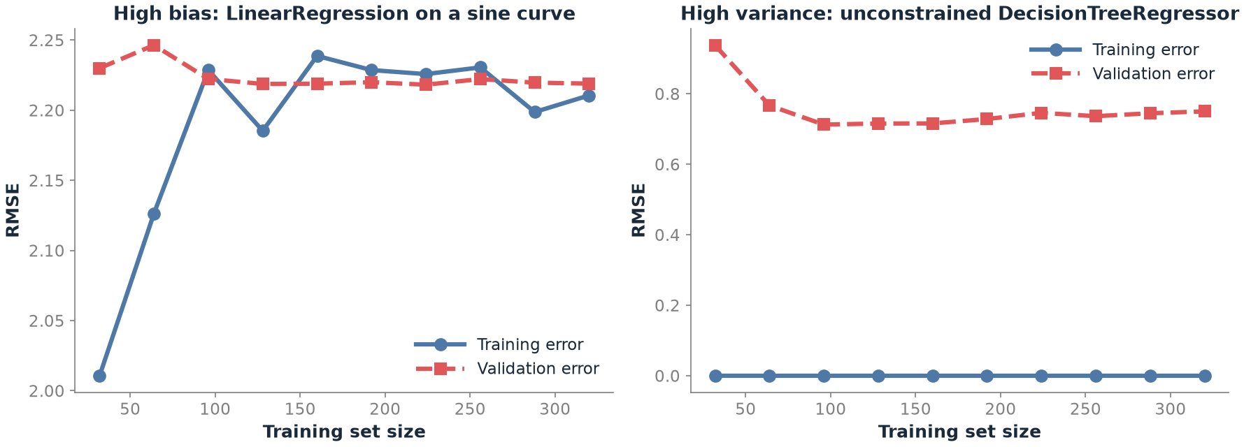
Figure 18.1 shows both failure modes side by side. On the left, LinearRegression’s training RMSE starts a touch lower, around 2.01 with the smallest training slice, then rises and settles alongside validation RMSE in a tight band, roughly 2.19 to 2.25, for the rest of the curve. Neither curve improves as more data arrives, and there’s no consistent gap between them: the signature of high bias, a model too simple to represent a sine curve no matter how much data it sees. On the right, the unconstrained decision tree’s training RMSE sits at nearly zero throughout. It memorises every training point exactly. Validation RMSE starts at 0.938, drops to around 0.71-0.75, and stays there: a gap that narrows a little, as the text above predicts, but never closes. That’s the signature of high variance.
18.2.3 L2 Regularisation (Ridge)
Ridge adds the sum of squared weights to the loss: , where controls penalty strength. This pushes gradient descent towards smaller weights across the board. Ridge shrinks every weight towards zero, but keeps every feature in the model. It’s the right choice when most features are believed useful, but noisy.
18.2.4 L1 Regularisation (Lasso)
Lasso adds the sum of absolute weights instead: . The geometric reason Lasso behaves differently from Ridge is subtle. The L1 penalty’s constraint region has corners exactly on the axes. When the constrained solution lands on one of those corners, a weight is driven to exactly zero. The L1 penalty has no gradient at zero, so scikit-learn fits Lasso by coordinate descent, not gradient descent. Lasso therefore produces sparse solutions. It zeros out irrelevant features, making it a form of automatic feature selection that Ridge structurally cannot do.
18.2.5 Elastic Net
Elastic Net combines both penalties: , as scikit-learn writes it. scikit-learn also scales the data-fit term by for Lasso and Elastic Net, but not for Ridge. So the same means a different strength in each of the three. It gets Lasso’s sparsity while handling correlated features more gracefully. Lasso tends to pick one feature from a correlated group arbitrarily and zero out the rest. Elastic Net tends to keep or drop correlated groups together instead.
18.2.6 Dropout (Neural Networks)
During each training step, dropout randomly zeroes a fraction of neurons, preventing them from co-adapting into a fixed, fragile pattern. Any given neuron has to be independently useful, not just useful as part of one specific combination. During training, frameworks such as PyTorch scale the surviving activations up by , where is the dropout rate. That keeps the expected activation the same, so at inference every neuron is active and no scaling is needed. A dropout rate of 0.2-0.5 is typical. It’s one of the most commonly used regularisers for deep networks.
18.2.7 Early Stopping
Monitor validation loss during training. Stop once it hasn’t improved for a set number of epochs, the patience, even while training loss keeps falling. Validation loss is noisy, so a single rise isn’t enough. Patience catches the point where overfitting has set in. It’s simple, effective, and nearly free in compute terms. It’s just stopping a run early.
18.3 Trade-offs and Limits
Too much regularisation ( too high) underfits. The model can’t capture the real signal, and both training and test performance suffer together. Too little ( too low, or none) overfits. Training error is low but test error is high. A widening gap between the two is the real symptom. The sweet spot is found by cross-validated search over : RidgeCV, LassoCV, or the general hyperparameter search machinery from Chapter 17.
18.4 Procedures
Procedure 18.1 (Choose Between Ridge, Lasso, and Elastic Net). When to use: selecting a regularisation strategy for a linear model.
# Want automatic feature selection (some weights -> exactly 0)?
# No  -> Ridge (L2): keeps all features, shrinks them
# Yes -> features correlated with each other?
#        Yes -> Elastic Net (handles correlated groups better)
#        No  -> Lasso (L1)
Quick rule: start with Ridge; try Lasso if many features are suspected irrelevant; use Elastic Net when features are highly correlated.
Procedure 18.2 (Apply Ridge with Cross-Validated Alpha). When to use: the default regularised-regression starting point.
from sklearn.linear_model import RidgeCV
import numpy as np

ridge_cv = RidgeCV(alphas=np.logspace(-3, 3, 100), cv=5)
ridge_cv.fit(X_train_scaled, y_train)
print(f'Best alpha: {ridge_cv.alpha_}')
Procedure 18.3 (Apply Lasso and Count Eliminated Features). When to use: suspected irrelevant features, or automatic feature selection is wanted alongside regularisation.
from sklearn.linear_model import LassoCV

lasso_cv = LassoCV(
    alphas=np.logspace(-4, 1, 100), cv=5, max_iter=10000
)
lasso_cv.fit(X_train_scaled, y_train)
n_zero = (lasso_cv.coef_ == 0).sum()
n_total = len(lasso_cv.coef_)
print(
    f'{n_zero} of {n_total} features eliminated, '
    f'best alpha={lasso_cv.alpha_}'
)
Common mistake: forgetting to scale features before regularising. An unscaled feature on a much larger numeric range gets penalised unfairly relative to a small-scale one, since the penalty is applied to the raw weight magnitude. Always StandardScaler() first.
Procedure 18.4 (Apply Regularised Logistic Regression). When to use: classification with the same overfitting risk.
from sklearn.linear_model import LogisticRegressionCV

# C is the inverse of alpha: smaller C = more regularisation
lr_l2 = LogisticRegressionCV(
    Cs=20, cv=5, max_iter=1000,  # L2 is the default penalty
)
lr_l2.fit(X_train_scaled, y_train)
Procedure 18.5 (Diagnose Bias vs. Variance with a Learning Curve). When to use: deciding whether “get more data” or “add regularisation, or a simpler model” is the right next step, before spending time or money on either.
from sklearn.model_selection import learning_curve
import numpy as np

train_sizes, train_scores, val_scores = learning_curve(
    estimator, X_train, y_train,
    train_sizes=np.linspace(0.1, 1.0, 10),
    cv=5, scoring='neg_root_mean_squared_error',
)

train_rmse = -train_scores.mean(axis=1)
val_rmse = -val_scores.mean(axis=1)

plt.plot(train_sizes, train_rmse, label='Training error')
plt.plot(train_sizes, val_rmse, label='Validation error')
plt.xlabel('Training set size')
plt.ylabel('RMSE')
plt.legend()
Common mistake: reading the curve at a single training-set size instead of its overall shape. The diagnostic signal is whether the gap between the two curves narrows as size increases, not the error at any one point on its own.
18.5 Worked Example
Fitting a degree-15 polynomial to 60 noisy points generated from a simple quadratic ( plus Gaussian noise), with a 70/30 train/test split, produces the textbook overfitting shape:
import numpy as np
from sklearn.model_selection import train_test_split
from sklearn.preprocessing import PolynomialFeatures, StandardScaler
from sklearn.linear_model import LinearRegression

rng = np.random.RandomState(42)
X = rng.uniform(-5, 5, 60).reshape(-1, 1)
y = 0.5 * X.ravel()**2 - X.ravel() + 2 + rng.normal(0, 2, 60)

X_train, X_test, y_train, y_test = train_test_split(
    X, y, test_size=0.3, random_state=42
)

poly = PolynomialFeatures(degree=15, include_bias=False)
scaler = StandardScaler()
X_train_poly = scaler.fit_transform(poly.fit_transform(X_train))
X_test_poly = scaler.transform(poly.transform(X_test))

lr = LinearRegression().fit(X_train_poly, y_train)
Measured: unregularised, this model reaches training RMSE 1.412 but test RMSE 1.912, about 35% worse on data it hasn’t seen. That’s a real but modest overfitting gap, given how small this dataset is (42 training points). Applying RidgeCV (best ) brings test RMSE down to 1.461, below even its own training RMSE of 1.819. The regularised model generalises better than it fits, the opposite of the unregularised model’s pattern. LassoCV (best ) does comparably well on test RMSE (1.455, the best of the three), while additionally zeroing out 11 of the 15 polynomial-feature coefficients entirely. Lasso didn’t just shrink the overfit away. It explicitly decided most of the degree-15 expansion’s terms weren’t worth keeping, leaving a much smaller model behind that generalises better than the 15-term original it started from, even without recovering the exact quadratic shape.
This is the bias-variance trade-off made concrete. Both Ridge and Lasso accept worse training fit than the unregularised model (RMSE 1.819 and 1.793 vs. 1.412), in exchange for better test performance (1.461 and 1.455 vs. 1.912). That’s a deliberate increase in bias that gets a larger reduction in variance, exactly as the Bias-Variance Trade-off section predicts.
from sagemaker.linear_learner import LinearLearner

ll = LinearLearner(
    predictor_type='binary_classifier',
    l1=0.01,    # L1 regularisation strength
    wd=0.001,   # weight decay = L2 regularisation
)
When to prefer SageMaker Linear Learner: when the regularised linear model needs to be trained at a scale beyond a single machine’s memory, or deployed as a managed endpoint without hand-building the serving infrastructure. For the polynomial-overfitting scale in this chapter’s Worked Example, a local scikit-learn pipeline is simpler and faster.
18.6 History and Further Reading
Murphy’s Introduction, Ch. 13, gives the full mathematical treatment of L1, L2, and Elastic Net (Murphy 2022). Burkov, Ch. 4, explains regularisation accessibly with visuals (Burkov 2019). Géron’s Hands-On Machine Learning, Ch. 4, works through Ridge, Lasso, and Elastic Net side by side in code, including the geometric picture of why Lasso zeroes out coefficients and Ridge only shrinks them (Géron 2019). Bishop’s Pattern Recognition and Machine Learning, Ch. 3, gives the probabilistic interpretation (L2 as a Gaussian prior, L1 as a Laplace prior) (Bishop 2006).
18.7 How This Connects
This chapter builds on Chapter 4’s calculus and optimisation (regularisation modifies the loss function being optimised) and Chapter 13’s cross-validation (needed to choose properly). It enables the dropout and weight-decay techniques Book 2, Chapter 28 applies to neural networks, where L2 regularisation reappears under the name “weight decay.” It’s often confused with feature selection (Chapter 15). L1 regularisation does perform feature selection as a side effect, but Chapter 15 covers the explicit, dedicated methods for it.
18.8 Exercises
[W] Explain in your own words why Ridge shrinks weights towards zero without ever setting them exactly to zero, while Lasso can.
[W] A model shows training RMSE 1.2 and test RMSE 3.1. State whether this is a bias problem or a variance problem, and name one regularisation technique that would help.
[A] Using Listing 18.7’s measured numbers, compute the ratio of test RMSE to train RMSE for the unregularised model (1.912/1.412) and for the Ridge model (1.461/1.819), and explain what a ratio below 1.0 shows about the Ridge model’s fit.
[A] Using Listing 18.4’s pattern, explain why Lasso zeroing 11 of 15 polynomial coefficients is broadly consistent with the true underlying relationship being quadratic (degree 2, i.e. needing only 2 non-trivial polynomial terms beyond the intercept), even though a few extra nonzero terms remain, likely absorbing noise from a training set of only 42 points.
[E] A colleague sets
alpha=100for a Ridge model “to be safe against overfitting” without cross-validating it. Using this chapter’s Trade-offs section, explain what’s likely to go wrong.[E] A teammate regularises a model with features on wildly different scales (one column in the thousands, another between 0 and 1) without scaling first. Using Procedure 18.3’s common mistake, predict what will happen to the two features’ effective regularisation strength.
[R] Read the Bishop (Pattern Recognition and Machine Learning) Ch. 3 treatment of L2 as a Gaussian prior. Explain, in your own words, how choosing a smaller prior variance corresponds to a larger in the Ridge loss function.
18.9 Mental Model
Regularisation is Occam’s Razor applied to machine learning. Among models that explain the data equally well, prefer the simpler one. The penalty term is a formal, tunable statement of that preference. controls exactly how strongly simplicity is preferred over fit. Turn the dial too low and the model memorises noise. Turn it too high and the model can’t see the signal.