Chapter 11
Supervised Learning: Overview of Approaches
Every supervised learning algorithm does the same thing. It takes examples where the answer is already known (this tumour was malignant, this customer churned, this house sold for $420k). It learns a mapping from inputs to outputs that generalises to examples it hasn’t seen. Dozens of algorithm families claim to solve it, each with a different idea of what that mapping should look like. No one algorithm wins every time. This chapter provides an overview of these algorithms: what the major families assume, where each one excels, and the trade-off, bias versus variance, that explains why picking an algorithm is picking a set of assumptions about your data.
11.1 Motivation
A Solutions Architect doesn’t need to have implemented every algorithm from scratch. But they do need enough working knowledge to answer a very practical question fast: given this dataset and this business constraint, what’s the first thing worth trying? Reaching for the wrong family costs time. A KNN model that can’t serve predictions inside a latency budget. A decision tree that overfits the moment it touches data. A linear model fit to a relationship that curves: wrong in the same way no matter how much data arrives. Every algorithm family encodes an inductive bias: an assumption about the shape of the relationship between inputs and outputs. There’s no assumption-free algorithm. Choosing one is choosing what you’re willing to believe about your data. Flexibility has its own cost. A neural network trained on 800 rows will usually lose to a logistic regression trained in a couple of minutes on the same data. Not because the network’s assumptions are wrong. It barely has any. But 800 rows isn’t enough data to pin down such an unconstrained model. Book 2 covers exactly why, once neural networks have been introduced.
11.2 Exposition
11.2.1 The Bias-Variance Trade-Off
This is probably the most important idea in supervised learning. Everything else in this chapter is downstream of it. Every model’s error comes from two sources.
Bias is how wrong the model’s assumptions are. Systematically. No matter how much data it gets. A linear model fit to a curved relationship stays wrong forever. More data doesn’t fix a mismatched hypothesis class. It just makes the wrongness more precisely measured.
Variance is how much the model’s predictions change when trained on a different sample from the same population. A model that memorises its training data exactly will produce a completely different fit if a handful of training examples change. That instability is variance.
The irreducible error is noise in the data. No model removes it. The trade-off is between the other two. A simple model (a straight line) has high bias and low variance. It’s wrong in the same way every time, but it’s stable. A flexible model (an unpruned decision tree) has low bias and high variance. It can better represent the true relationship. But it also happily fits noise, and small changes in training data produce a very different fit. Model complexity is a dial. The goal is finding where on that dial test error is minimised. That point has to be found empirically, because it depends on the specific dataset. Chapter 13 (Cross-Validation & Model Selection) is the tool that finds it.
11.2.2 Linear Models
What they assume: the relationship between inputs and output is a straight line (regression) or that a hyperplane can separate the classes (classification).
A hyperplane is the general-dimensional version of a line. In two dimensions it’s an ordinary line. In three, an ordinary flat plane. In dimensions, it’s whatever flat, one-dimension-lower surface generalises that idea. It’s defined by the same equation either way: , using the dot product from Chapter 3. Every point on one side of that surface gives . Every point on the other side gives a negative value. A linear classifier’s whole job is choosing and so that surface falls between the two classes as cleanly as possible. A dataset with 30 features doesn’t live somewhere a hyperplane can be drawn and looked at. But the equation that defines one doesn’t care how many dimensions it’s operating in.
Logistic Regression is a classifier despite the name. It models with a sigmoid applied to a linear combination of features, and its outputs are probabilities, not just labels, and often reasonably well calibrated ones.
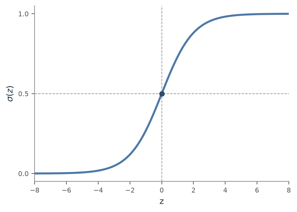
The sigmoid function is , and its job is squashing any real number into the open interval , so it can be read as a probability. Large positive pushes towards 1; large negative pushes it towards 0; gives exactly 0.5. Plotted, it’s a smooth S-shaped curve (Figure 11.1), steep near the middle and flat at both ends. That flatness matters: once the model is already confident, a further change to its linear combination of features barely moves the predicted probability, but near , a small change swings the prediction hard in one direction or the other.
Linear Regression fits a line by minimising squared error. Both are fast, interpretable (the coefficients are the explanation), and a recommended first step. Train the linear baseline before anything fancier. If a complex model can’t beat your baseline, the problem is the features or the data, not the missing complexity. Weaknesses: no nonlinear relationships without manual feature engineering, sensitivity to outliers (linear regression), and unstable coefficients when features are strongly correlated with each other (multicollinearity), which regularisation only partly fixes.
Regularisation adds a penalty for complexity to what a model is trying to minimise, on top of prediction error. Instead of fitting the training data as closely as possible, the model is pushed towards smaller, simpler coefficients, which tends to generalise better and lean less heavily on any single feature. For linear regression, that means adding a cost for large weights to the loss function, so a handful of correlated features can’t each grab an oversized, unstable share of the prediction the way they could unregularised. It doesn’t remove the correlation. It just limits the damage. Chapter 18 covers regularisation properly, including its two standard forms, Ridge and Lasso, and why they behave differently.
11.2.3 Support Vector Machines
What they assume: among every hyperplane that separates the classes, the one with the widest margin to the nearest points of each class generalises best.
A Support Vector Machine (SVM) starts from the same hyperplane idea as Logistic Regression, but picks it differently. Instead of any separating hyperplane, it finds the one maximising the distance to the closest point of either class, the margin. Only those closest points, the support vectors, determine where the boundary sits. Every other point could move, or vanish, without changing the decision boundary at all. Real data is rarely perfectly separable, so a slack parameter trades margin width against tolerating some misclassified or margin-violating points. Small gives a wide margin that tolerates more violations: higher bias, lower variance. Large gives a narrow margin that tolerates few: lower bias, higher variance. That’s the same trade-off this chapter’s first section named.
A kernel function computes the dot product two points would have after being mapped into some higher-dimensional space, without ever performing that mapping explicitly. That matters because a boundary that’s a curve in the original space can be a hyperplane in the right higher-dimensional one. SVM training only ever needs dot products between points, never their raw transformed coordinates. The RBF kernel, , corresponds to an infinite-dimensional mapping and is the default choice when there’s no reason to assume a specific functional form. This is exactly the trick that lets an SVM draw a curved boundary around data no straight line can separate, the concentric-circles case later in this chapter’s Worked Example, where Logistic Regression collapses to 0.289.
SVMs handle high-dimensional data well, and remain effective even when the number of features exceeds the number of rows. But training scales poorly past roughly tens of thousands of rows. And, like every distance-based method in this chapter, they need scaled features to behave sensibly.
11.2.4 Tree-Based Models
What they assume: the relationship is well-approximated by a sequence of if/else splits on individual features.
A Decision Tree recursively splits training data on whichever feature best separates classes, or reduces regression error, at each node. Each leaf is a prediction. Trees are naturally interpretable (print one and read it like a flowchart) and need no feature scaling. (scikit-learn’s trees still need categories encoded as numbers.) Their weakness is the high-variance failure mode above: an unconstrained tree memorises its training set, and a small change in the data produces a structurally different tree. Ensembling many trees, covered in Chapter 12, is the standard fix and the reason trees remain the dominant building block for tabular data despite being weak individually.
11.2.5 Distance-Based Models
What they assume: similar inputs produce similar outputs: nearby points in feature space share a label.
k-Nearest Neighbours (KNN) classifies a new point by finding its closest training examples, Euclidean distance by default, and taking a majority vote. For regression, it averages their targets. KNN makes no assumption about the shape of the boundary. It can represent arbitrarily complex relationships. But it pays for that flexibility at prediction time: every prediction requires computing distance to every training point, an cost per prediction that gets expensive fast. It also degrades in high dimensions: the curse of dimensionality. As dimensionality grows, all points become roughly equidistant, and “nearest” loses meaning. And it requires feature scaling. Distance is meaningless when one feature ranges and another .
11.2.6 Probabilistic Models
What they assume: features are conditionally independent given the class label, the “naive” in Naive Bayes.
That assumption is almost never true, and the algorithm works well anyway. Naive Bayes applies Bayes’ theorem to compute the posterior probability of each class. The independence assumption reduces this to multiplying per-feature likelihoods, which is extremely fast to train and predict. It’s a strong, cheap baseline for text classification (it works well on bag-of-words features, even though words are far from independent) and for any problem with very little training data, since it has few parameters to estimate. It underestimates feature correlations and can’t represent interactions, so it’s rarely competitive as a final model. But as a five-minute sanity check, it’s hard to beat.
11.2.7 The No Free Lunch Theorem
There’s a formal result behind the intuition that “it depends.” Averaged over all possible problems, no algorithm outperforms any other, including random guessing. What this rules out is a universal favourite. What it does not rule out, and what makes data science a skill rather than a lookup table, is that specific algorithms reliably outperform others on the specific kinds of problems that show up in practice. On tabular data, gradient-boosted trees (Chapter 12) win most of the time. On unstructured data, deep learning wins. Neither fact contradicts No Free Lunch, because “tabular data” and “image data” are not uniform samples over all possible problems. They have structure, and different algorithms are built to exploit different kinds of structure.
11.3 Trade-offs and Limits
| Algorithm | Bias | Variance | Interpretable | Nonlinear | Speed |
|---|---|---|---|---|---|
| Logistic Regression | High | Low | Yes | No | Very fast |
| SVM (RBF kernel) | Low–Med | Low–Med | No | Yes | Slow to train at scale |
| Decision Tree (deep) | Low | High | Yes (if shallow) | Yes | Fast |
| KNN | Low | High | No | Yes | Slow at predict time |
| Naive Bayes | High | Low | Partial | No | Very fast |
| Random Forest | Low–Med | Low–Med | No | Yes | Medium |
No row in this table is dominant. That’s the No Free Lunch theorem showing up as a design constraint. The practical resolution is empirical: try the fast, interpretable baseline first, and let cross-validated performance decide whether the added complexity of a more flexible family gives you something useful.
11.4 Procedures
Procedure 11.1 (Train and Evaluate Any sklearn Classifier: the Universal Pattern). When to use: every classification task, regardless of algorithm: the API is identical across all five families above.
from sklearn.model_selection import train_test_split
from sklearn.preprocessing import StandardScaler
from sklearn.pipeline import Pipeline
# swap for any classifier
from sklearn.linear_model import LogisticRegression
from sklearn.metrics import accuracy_score, classification_report

X_train, X_test, y_train, y_test = train_test_split(
    X, y, test_size=0.2, random_state=RANDOM_SEED, stratify=y
)

clf = Pipeline([
    ('scaler', StandardScaler()),
    ('model', LogisticRegression(max_iter=1000))
])
clf.fit(X_train, y_train)
y_pred = clf.predict(X_test)

print(f'Accuracy: {accuracy_score(y_test, y_pred):.3f}')
print(classification_report(y_test, y_pred))
Why the Pipeline matters: it guarantees the scaler is fitted only on training data and applied, not refitted, on test data. Fitting the scaler on the full dataset before splitting is a leakage bug, the classification analogue of the leakage failure mode from Chapter 2.
Procedure 11.2 (Compare Multiple Classifiers Under Identical Conditions). When to use: deciding which algorithm family is worth investing tuning time in, before committing to one.
from sklearn.model_selection import cross_val_score

classifiers = {
    'Logistic Regression': LogisticRegression(max_iter=1000),
    'Decision Tree': DecisionTreeClassifier(
        random_state=RANDOM_SEED
    ),
    'K-Nearest Neighbours': KNeighborsClassifier(n_neighbors=5),
    'Naive Bayes': GaussianNB(),
    'Random Forest': RandomForestClassifier(
        random_state=RANDOM_SEED, n_estimators=100
    ),
    'SVM (RBF)': SVC(random_state=RANDOM_SEED),
}

for name, clf in classifiers.items():
    pipe = Pipeline([('scaler', StandardScaler()), ('clf', clf)])
    scores = cross_val_score(
        pipe, X_train, y_train, cv=5, scoring='accuracy'
    )
    print(f'{name:<25} {scores.mean():.3f} ± {scores.std():.3f}')
Common mistake: comparing algorithms using a single train/test split. Different splits can reorder the ranking entirely on a small dataset. Chapter 13 quantifies exactly how much.
Procedure 11.3 (Get and Threshold Prediction Probabilities). When to use: whenever a confidence score matters more than a hard label: risk scoring, ranking, or a business-specific decision threshold (the precision/recall trade-off from Chapter 2).
proba = clf.predict_proba(X_test)   # shape (n_samples, n_classes)
positive_class_proba = proba[:, 1]

threshold = 0.3   # lower than 0.5 → higher recall, lower precision
y_pred_custom = (positive_class_proba >= threshold).astype(int)
Not every estimator supports predict_proba (LinearSVC is a common exception). Use decision_function() instead, or switch to SVC(probability=True).
Procedure 11.4 (Diagnose Bias vs. Variance from the Train/Test Gap). When to use: a model’s cross-validated score is disappointing and the next step, more data, more regularisation, or a more flexible model, depends on which failure mode is present.
train_acc = accuracy_score(y_train, clf.predict(X_train))
test_acc  = accuracy_score(y_test, clf.predict(X_test))
gap = train_acc - test_acc
print(
    f'Train: {train_acc:.3f}  Test: {test_acc:.3f}  Gap: {gap:.3f}'
)
Rule of thumb: train high, test low, large gap → high variance (overfitting): simplify the model or get more data. Train and test both low → high bias (underfitting): use a more flexible model or better features. Wide spread across CV folds → high variance regardless of the train/test gap.
11.5 Worked Example
The tutorial notebook runs six classifiers (Logistic Regression, SVM, Decision Tree, KNN, Naive Bayes, Random Forest) on the sklearn breast cancer dataset. It has 569 tumour samples and 30 numeric features, labelled malignant (class 0) or benign (class 1), split 62.7% benign / 37.3% malignant. A stratified 80/20 split gives 455 training and 114 test samples.
Benchmarking all six with Procedure 11.2 (5-fold CV on the training set) plus a held-out test score and timing gives the results below. Timings are from this machine and vary by run and hardware. The CV and test scores are deterministic given the fixed seed.
| Algorithm | Test Acc. | CV Mean ± Std | Train Time | Predict Time |
|---|---|---|---|---|
| Logistic Regression | 0.982 | 0.980 ± 0.013 | 16.0 ms | 1.1 ms |
| SVM (RBF) | 0.982 | 0.971 ± 0.018 | 6.5 ms | 1.5 ms |
| K-Nearest Neighbours | 0.956 | 0.967 ± 0.021 | 1.5 ms | 35.4 ms |
| Random Forest | 0.956 | 0.954 ± 0.023 | 95.7 ms | 5.8 ms |
| Naive Bayes | 0.930 | 0.932 ± 0.004 | 1.7 ms | 0.6 ms |
| Decision Tree | 0.912 | 0.910 ± 0.019 | 7.8 ms | 0.9 ms |
Logistic Regression and SVM tie for the top test accuracy. That’s unsurprising: 30 well-engineered clinical features separating two tumour classes is close to the linear-model sweet spot. The RBF kernel’s added flexibility here doesn’t help beyond what a straight hyperplane was already finding. Its slightly lower CV mean (0.971 vs. 0.980) hints at a marginally less stable fit for capacity the data didn’t need. Two details are worth more attention than the ranking. First, KNN’s prediction time (35.4 ms) dwarfs every other model’s: more than six times slower than the next-slowest, Random Forest (5.8 ms), and over sixty times slower than the fastest, Naive Bayes (0.6 ms). That’s the cost from the Exposition section, visible directly in milliseconds rather than asserted. Second, Naive Bayes has by far the lowest CV standard deviation (±0.004 against ±0.013–0.023 for everything else). The independence assumption gives it less to overfit, trading a slightly lower mean for a much more stable estimate: exactly the low-variance side of the bias-variance table.
Random Forest’s full classification report on the held-out test set (with all 30 features) reads: malignant precision 0.95, recall 0.93, f1 0.94 (support 42); benign precision 0.96, recall 0.97, f1 0.97 (support 72); overall accuracy 0.96. The confusion matrix is [[39, 3], [2, 70]]: 3 malignant tumours misclassified as benign, 2 benign misclassified as malignant. The costlier error clinically, a missed malignancy, is the more common one here: 3 against 2. That’s exactly why Chapter 2’s point about business-owned thresholds matters, even on a textbook dataset.
Restricting every classifier to two features (mean radius, mean texture) so the decision boundary can be plotted in 2D drops accuracy across the board. Logistic Regression, KNN, and Naive Bayes all land at 0.877, Random Forest at 0.860, and Decision Tree falls hardest, to 0.789. The interesting result isn’t the accuracy drop: that’s expected, since 28 informative features were discarded. It’s that three structurally different algorithms converge on the same accuracy with only two features. The tree, the algorithm best able to exploit many features via deep splits, suffers the most from losing them, since it has nothing left to split on beyond two axes.
Finally, a direct empirical example of No Free Lunch: on a synthetic dataset of two linearly-separable blob clusters, both Logistic Regression and Random Forest score a perfect 1.000. On a synthetic dataset of two concentric circles, no linear boundary can separate them, Random Forest still scores 1.000. Logistic Regression collapses to 0.289. That’s worse than the ~0.5 a coin flip would give on balanced classes. With features standardised around the same origin the two circles share, the linear decision boundary lands on the wrong side of the split, actively anti-correlating with the true label rather than merely failing to find one. Two algorithms, two datasets, and the ranking flips completely. The No Free Lunch theorem is not an abstraction here. It’s a number that goes from 1.000 to 0.289 depending on the shape of the data.
11.6 History and Further Reading
Burkov’s Chapter 3 gives a concise, precise pass through the main algorithm families this chapter covers. Chapter 4 formalises “the anatomy of a learning algorithm,” the representation/loss/optimisation breakdown this chapter’s Motivation section leans on (Burkov 2019). Murphy’s Introduction, Chapters 9–10, gives the full probabilistic treatment of linear and logistic regression for readers who want the derivations behind the sigmoid and the squared-error loss (Murphy 2022). Géron’s Hands-On Machine Learning devotes separate chapters to classification (Ch. 3), support vector machines (Ch. 5), and decision trees (Ch. 6), each with worked Scikit-Learn code for the families this chapter surveys (Géron 2019). The supervised-learning No Free Lunch theorem is due to Wolpert (1996). Wolpert and Macready (1997) proved the companion result for optimisation. It’s worth reading in the original for how narrow its actual claim is: far narrower than the popular one-line summary suggests.
11.7 How This Connects
This chapter builds on Chapter 3 (the probability and linear algebra underneath every algorithm here), Chapter 6 (the Python/sklearn ecosystem all the code above assumes), and Chapter 10 (the lifecycle stage this sits inside). It enables Chapter 12, where these same algorithms (trees especially) become base learners inside ensembles, and Chapter 16, which needs trained models before it can evaluate them. It’s often confused with the supervised/unsupervised distinction: everything in this chapter learns from labelled examples. Chapter 19 covers what happens when there’s no label to learn from at all.
11.8 Exercises
[W] For each of the following, name the algorithm family (Linear, Support Vector Machine, Tree-Based, Distance-Based, Probabilistic) and state its core assumption in one sentence: (a) spam detection using word-count features; (b) predicting house price from square footage and location; (c) classifying flowers from petal measurements using their five closest labelled neighbours.
[W] Explain, in your own words, why increasing model flexibility (e.g., letting a decision tree grow deeper) tends to reduce bias while increasing variance. Use the bias-variance equation from this chapter.
[A] Using the benchmark table in the Worked Example, identify every algorithm whose test accuracy exceeds its CV mean accuracy. Explain what that ordering does, or doesn’t, tell you about overfitting for those models.
[A] The Worked Example shows Decision Tree accuracy falling from 0.912 (30 features) to 0.789 (2 features), the largest drop of any algorithm. Using this chapter’s description of how trees split, explain why restricting to two features hurts a tree more than it hurts Naive Bayes (0.930 → 0.877).
[E] A client has a 40,000-row tabular dataset with strongly nonlinear feature interactions and needs predictions to run inside a 5ms latency budget per request. Using Listing 11.1 and this chapter’s Trade-offs table, name the algorithm you would rule out first, and explain why using the prediction-time numbers from the Worked Example.
[E] The No Free Lunch theorem is often summarised as “no algorithm is better than any other.” Using the blobs-vs-circles result (1.000 vs. 0.289 for Logistic Regression), explain why that popular summary is misleading for a working data scientist, and state the narrower claim the theorem makes.
[R] Read Burkov’s Chapter 4 on the anatomy of a learning algorithm. Apply its three-part framework (hypothesis representation, loss function, optimisation procedure) to Naive Bayes, and explain what makes its optimisation step so much faster than logistic regression’s.
11.9 Mental Model
Every supervised learning algorithm is a machine for turning labelled examples into a decision rule. The algorithms differ only in what shape of rule they’re willing to consider: a line, a maximum-margin boundary (straight or kernel-bent), a set of rectangular cuts, a neighbourhood vote, a product of per-feature likelihoods. Before touching code, ask what shape the real boundary between classes (or the true curve through the regression data) is likely to take. The answer to that question picks the first algorithm to try faster than any benchmark table can.